4.4.7. State-Space Representation and Integration with OpenFAST
4.4.7.1. State, Constraint, Input, and Output Variables
The OLAF module has been integrated into the latest version of OpenFAST via AeroDyn, following the OpenFAST modularization framework ([olaf-Jon13, olaf-SJJ15]). To follow the OpenFAST framework, the vortex code is written as a module, and its formulation comprises state, constraint, and output equations. The data manipulated by the module include the following vectors: constant parameters, \(\vec{p}\); inputs, \(\vec{u}\); constrained state, \(\vec{z}\); states, \(\vec{x}\); and outputs, \(\vec{y}\). The vectors are defined as follows:
Parameters, \(\vec{p}~-\) a set of internal system values that are independent of the states and inputs. The parameters can be fully defined at initialization and characterize the system state and output equations.
Inputs, \(\vec{u}~-\) a set of values supplied to the module that, along with the states, are needed to calculate future states and the system output.
Constraint states, \(\vec{z}~-\) algebraic variables that are calculated using a nonlinear solver, based on values from the current time step.
States, \(\vec{x}~-\) a set of internal values of the module. They are influenced by the inputs and used to calculate future state values and output. Continuous states are employed, meaning that the states are differentiable in time and characterized by continuous time-differential equations.
Outputs, \(\vec{y}~-\) a set of values calculated and returned by the module that depend on the states, inputs, and/or parameters through output equations.
The parameters of the vortex code include:
Fluid characteristics: kinematic viscosity, \(\nu\).
Airfoil characteristics: chord \(c\) and polar data – \(C_l(\alpha)\), \(C_d(\alpha)\), \(C_m(\alpha)\)).
Algorithmic methods and parameters, e.g., regularization, viscous diffusion, discretization, wake geometry, and acceleration.
The inputs of the vortex code are:
Position, orientation, translational velocity, and rotational velocity of the different nodes of the lifting lines (\(\vec{r}_{ll}\), \(\Lambda_{ll}\), \(\vec{\dot{r}}_{ll}\), and \(\vec{\omega}_{ll}\), respectively), gathered into the vector, \(\vec{x}_{\text{elast},ll}\), for conciseness. These quantities are handled using the mesh-mapping functionality and data structure of OpenFAST.
Disturbed velocity field at requested locations, written \(\vec{V}_0=[\vec{V}_{0,ll}, \vec{V}_{0,m}]\). Locations are requested for lifting-line points, \(\vec{r}_{ll}\), and Lagrangian markers, \(\vec{r}_m\). Based on the parameters, this disturbed velocity field may contain the following influences: freestream, shear, veer, turbulence, tower, and nacelle disturbance. The locations where the velocity field is requested are typically the location of the Lagrangian markers.
The constraint states are:
The circulation intensity along the lifting lines, \(\Gamma_{ll}\).
The continuous states are:
The position of the Lagrangian markers, \(\vec{r}_m\)
The vorticity associated with each vortex element, \(\vec{\omega}_e\). For a projection of the vorticity onto vortex segments, this corresponds to the circulation, \(\vec{\Gamma}_e\). For each segment, \(\vec{\Gamma}_e= \Gamma_e \vec{dl}_e =\vec{\omega}_e dV_e\), with \(\vec{dl}_e\) and \(dV_e\), the vortex segment length and its equivalent vortex volume.
The outputs are 1:
The induced velocity at the lifting-line nodes, \(\vec{v}_{i,ll}\)
The locations where the undisturbed wind is computed, \(\vec{r}_{r}\) (typically \(\vec{r_{r}}=\vec{r}_m\)).
4.4.7.2. State, Constraint, and Output Equations
An overview of the states, constraints, and output equations is given here. More details are provided in Section 4.4.6. The constraint equation is used to determine the circulation distribution along the span of each lifting line. For the van Garrel method, this circulation is a function of the angle of attack along the blade and the airfoil coefficients. The angle of attack at a given lifting-line node is a function of the undisturbed velocity, \(\vec{v}_{0,ll}\), and the velocity induced by the vorticity, \(\vec{v}_{i,ll}\), at that point. Part of the induced velocity is caused by the vorticity being shed and trailed at the current time step, which in turn is a function of the circulation distribution along the lifting line. This constraint equation may be written as:
where \(\vec{\Gamma}_p\) is the function that returns the circulation along the blade span, according to one of the methods presented in Section 4.4.6.3.
The state equation specifies the time evolution of the vorticity and the convection of the Lagrangian markers:
Here,
\(\vec{v}_\omega\) is the velocity induced by the vorticity in the domain;
\(\vec{V}_\omega(\vec{r},\vec{r}_m,\vec{\omega})\) is the function that computes this induced velocity at a given point, \(\vec{r}\), based on the location of the Lagrangian markers and the intensity of the vortex elements;
the subscript \(e\) indicates that a quantity is applied to an element; and
the vorticity, \(\vec{\omega}\), is recovered from the vorticity of the vortex elements by means of discrete convolutions.
For vortex-segment simulations, the viscous-splitting algorithm is used, and the convection step (Eq. (4.31)) is the main state equation being solved for. The vorticity stretching is automatically accounted for, and the diffusion is performed a posteriori. The velocity function, \(\vec{V}_\omega\), uses the Biot-Savart law. The output equation is:
4.4.7.3. Integration with AeroDyn
The vortex code has been integrated as a submodule of the aerodynamic module of OpenFAST, AeroDyn. The data workflow between the different modules and submodules of OpenFAST is illustrated in Fig. 4.16. AeroDyn inputs such as BEM options (e.g., tip-loss factor), skew model, and dynamic inflow are discarded when the vortex code is used. The environmental conditions, tower shadow, and dynamic stall model options are used. This integration required a restructuring of the AeroDyn module to isolate the parts of the code related to tower shadow modeling, induction computation, lifting-line-forces computations, and dynamic stall. The dynamic stall model is adapted when used in conjunction with the vortex code to ensure the effect of shed vorticity is not accounted for twice. The interface between AeroDyn and the inflow module, InflowWind, was accommodated to include the additionally requested points by the vortex code.
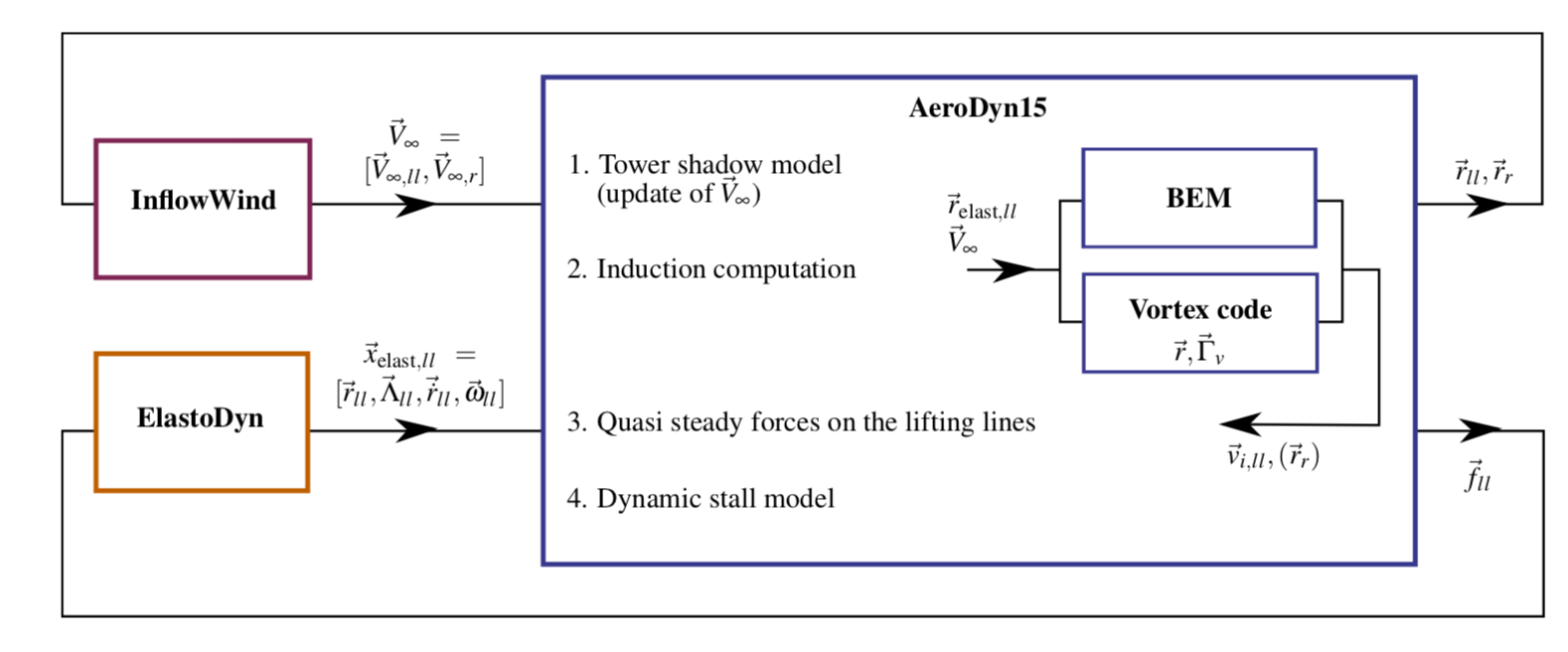
Fig. 4.16 OpenFAST-OLAF code integration workflow
- 1
The loads on the lifting line are not an output of the vortex code; their calculation is handled by a separate submodule of AeroDyn.