4.4.6. OLAF Theory
This section details the OLAF method and provides an overview of the computational method, followed by a brief explanation of its integration with OpenFAST.
4.4.6.1. Introduction - Vorticity Formulation
The vorticity equation for incompressible homogeneous flows in the absence of non-conservative force is given by Eq. (4.13)
Here, \(\vec{\omega}\) is the vorticity, \(\vec{u}\) is the velocity, and \(\nu\) is the viscosity. In free vortex wake methods, the vorticity equation is used to describe the evolution of the wake vorticity. Different approximations are introduced to ease its resolution, such as projecting the vorticity onto a discrete number of vortex elements (here vortex filaments), and separately treating the convection and diffusion steps, known as viscous-splitting. Several complications arise from the method; in particular, the discretization requires a regularization of the vorticity field (or velocity field) to ensure a smooth approximation.
The forces exerted by the blades onto the flow are expressed in vorticity formulation as well. This vorticity is bound to the blade and has a circulation associated with the lift force. A lifting-line formulation is used here to model the bound vorticity.
The different models of the implemented free vortex code are described in the following sections.
4.4.6.2. Discretization - Projection
The numerical method uses a finite number of states to model the continuous vorticity distribution. To achieve this, the vorticity distribution is projected onto basis function which is referred to as vortex elements. Vortex filaments are here used as elements that represents the vorticity field. A vortex filament is delimited by two points and hence assumes a direction formed by these two points. A vorticity tube is oriented along the unit vector \(\vec{e}_x\) of cross section \(dS\) and length \(l\). It can then be approximated by a vortex filament of length \(l\) oriented along the same direction. The total vorticity of the tube and the vortex filaments are the same and related by:
where \(\vec{\Gamma}\) is the circulation intensity of the vortex filament. If the vorticity tubes are complex and occupy a large volume, the projection onto vortex filaments is difficult and the projection onto vortex particle is more appropriate. Assuming the wake is confined to a thin vorticity layer which defines a velocity jump of know direction, it is possible to approximate the wake vorticity sheet as a mesh of vortex filaments. This is the basis of vortex filament wake methods. Vortex filaments are a singular representation of the vorticity field, as they occupy a line instead of a volume. To better represent the vorticity field, the filaments are “inflated”, a process referred to as regularization (see Section 4.4.6.8). The regularization of the vorticity field also regularizes the velocity field and avoids the singularities that would otherwise occur.
4.4.6.3. Lifting-Line Representation
The code relies on a lifting-line formulation. Lifting-line methods effectively lump the loads at each cross-section of the blade onto the mean line of the blade and do not account directly for the geometry of each cross-section. In the vorticity-based version of the lifting-line method, the blade is represented by a line of varying circulation. The line follows the motion of the blade and is referred to as “bound” circulation. The bound circulation does not follow the same dynamic equation as the free vorticity of the wake. Instead, the intensity is linked to airfoil lift via the Kutta-Joukowski theorem. Spanwise variation of the bound circulation results in vorticity being emitted into the wake. This is referred to as “trailed vorticity”. Time changes of the bound circulation are also emitted in the wake, referred to as “shed” vorticity. The subsequent paragraphs describe the representation of the bound vorticity.
4.4.6.3.1. Lifting-Line Panels and Emitted Wake Panels
The lifting-line and wake representation is illustrated in Fig. 4.15. The blade lifting-line is discretized into a finite number of panels, each of them forming a four sided vortex rings. The spanwise discretization follows the discretization of the AeroDyn blade input file. The number of spanwise panels, \(n_\text{LL}\), is one less than the total number of AeroDyn nodes, NumBlNds. The sides of the panels coincide with the lifting-line and the trailing edge of the blade. The lifting-line is currently defined as the 1/4 chord location from the leading edge (LE). More details on the panelling is provided in Section 4.4.6.3.2. At a given time step, the circulation of each lifting-line panel is determined according to one of the three methods developed in Section 4.4.6.3.3. At the end of the time step, the circulation of each lifting-line panel is emitted into the wake, forming free vorticity panels. To satisfy the Kutta condition, the circulation of the first near wake panel and the bound circulation are equivalent (see Fig. 4.15 b). The wake panels model the thin shear layer resulting from the continuation of the blade boundary layer. This shear layer can be modelled using a continuous distribution of vortex doublets. A constant doublet strength is assumed on each panel, which in turn is equivalent to a vortex ring of constant circulation.
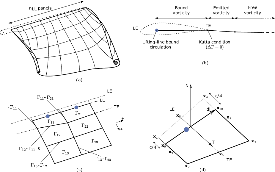
Fig. 4.15 Wake and lifting-line vorticity discretized into vortex ring panels. (a) Overview. (b) Cross-sectional view, defining the leading-edge, trailing edge, and lifting-line. (c) Circulation of panels and corresponding circulation for vorticity segments between panels. (d) Geometrical quantities for a lifting-line panel.
The current implementation stores the positions and circulations of the panel corner points. In the vortex ring formulation, the boundary between two panels corresponds to a vortex segment of intensity equal to the difference of circulation between the two panels. The convention used to define the segment intensity based on the panels intensity is shown in Fig. 4.15 c. Since the circulation of the bound panels and the first row of near wake panels are equal, the vortex segments located on the trailing edge have no circulation.
4.4.6.3.2. Panelling
The definitions used for the panelling of the blade are given in Fig. 4.15 d, following the notations of van Garrel ([olaf-vG03]). The leading edge and trailing edge (TE) locations are directly obtained from the AeroDyn mesh. At two spanwise locations, the LE and TE define the corner points: \(\vec{x}_1\), \(\vec{x}_2\), \(\vec{x}_3\), and \(\vec{x}_4\). The current implementation assumes that the aerodynamic center, the lifting-line, and the 1/4 chord location all coincide. For a given panel, the lifting-line is then delimited by the points \(\vec{x}_9= 3/4\,\vec{x}_1 + 1/4\, \vec{x}_2\) and \(\vec{x}_{10}=3/4\,\vec{x}_4 + 1/4\, \vec{x}_3\). The mid points of the four panel sides are noted \(\vec{x}_5\), \(\vec{x}_6\), \(\vec{x}_7\), and \(\vec{x}_8\). The lifting-line vector (\(\vec{dl}\)) as well as the vectors tangential (\(\vec{T}\)) and normal (\(\vec{N}\)) to the panel are defined as:
The area of the panel is obtained as \(dA = |(\vec{x}_6-\vec{x}_8)\times(\vec{x}_{7}-\vec{x}_5)|\). For CircSolvMethod=[1], the control points are located on the lifting-line at the location \(\vec{x}_9+\eta_j \vec{dl}\). The factor \(\eta_j\) is determined based on the full-cosine approximation of van Garrel. This is based on the spanwise widths of the current panel, \(w_j\), and the neighboring panels \(w_{j-1}\) and \(w_{j+1}\):
For an equidistant spacing, this discretization places the control points at the middle of the lifting-line (\(\eta=0.5\)). Theoretical circulation results for an elliptic wing with a cosine spacing are retrieved with such discretization since it places the control points closer to stronger trailing segments at the wing extremities (see e.g. [olaf-Ker00]).
4.4.6.3.3. Circulation Solving Methods
Three methods are implemented to determine the bound circulation strength. They are selected using the input CircSolvMethod, and are presented in the following sections.
4.4.6.3.3.1. Cl-Based Iterative Method
The Cl-based iterative method determines the circulation within a nonlinear iterative solver that makes use of the polar data at each control point located on the lifting line. The algorithm ensures that the lift obtained using the angle of attack and the polar data matches the lift obtained with the Kutta-Joukowski theorem. At present, it is the preferred method to compute the circulation along the blade span. It is selected with CircSolvMethod=[1]. The method is described in the work from van Garrel ([olaf-vG03]). The algorithm is implemented in at iterative approach using the following steps:
The circulation distribution from the previous time step is used as a guessed circulation, \(\Gamma_\text{prev}\).
The velocity at each control points \(j\) is computed as the sum of the wind velocity, the structural velocity, and the velocity induced by all the vorticity in the domain, evaluated at the control point location.
\[\begin{aligned} \vec{v}_j = \vec{V}_0 - \vec{V}_\text{elast} + \vec{v}_{\omega,\text{free}} + \vec{v}_{\Gamma_{ll}} \end{aligned}\]\(\vec{v}_{\omega,\text{free}}\) is the velocity induced by all free vortex filaments, as introduced in Eq. (4.22) . The contribution of \(\vec{v}_{\Gamma_{ll}}\) comes from the lifting-line panels and the first row of near wake panels, for which the circulation is set to \(\Gamma_\text{prev}\)
The circulation for all lifting-line panels \(j\) is obtained as follows.
\[\begin{aligned} \Gamma_{ll,j} =\frac{1}{2} C_{l,j}(\alpha_j) \frac{\left[ (\vec{v}_j \cdot \vec{N})^2 + (\vec{v}_j \cdot \vec{T})^2\right]\,dA}{ \sqrt{\left[(\vec{v}_j\times \vec{dl})\cdot\vec{N}\right]^2 + \left[(\vec{v}_j\times \vec{dl})\cdot\vec{T}\right]^2} } %\label{eq:} ,\quad\text{with} \quad \alpha_j = \operatorname{atan}\left(\frac{\vec{v}_j\cdot\vec{N}}{\vec{v}_j \cdot \vec{T}} \right) \end{aligned}\]The function \(C_{l,j}\) is the lift coefficient obtained from the polar data of blade section \(j\) and \(\alpha_j\) is the angle of attack at the control point.
The new circulation is set using the relaxation factor \(k_\text{relax}\) (CircSolvRelaxation):
\[\begin{aligned} \Gamma_\text{new}= \Gamma_\text{prev} + k_\text{relax} \Delta \Gamma ,\qquad \Delta \Gamma = \Gamma_{ll} - \Gamma_\text{prev} %\label{eq:} \end{aligned}\]Convergence is checked using the criterion \(k_\text{crit}\) (CircSolvConvCrit):
\[\begin{aligned} \frac{ \operatorname{max}(|\Delta \Gamma|}{\operatorname{mean}(|\Gamma_\text{new}|)} < k_\text{crit} \end{aligned}\]If convergence is not reached, steps 2-5 are repeated using \(\Gamma_\text{new}\) as the guessed circulation \(\Gamma_\text{prev}\).
4.4.6.3.3.2. No-flow-through Method
A no-flow-through circulation solving method (sometimes called Weissinger-L-based method) might be implemented in the future ([olaf-BL94, olaf-Gup06, olaf-Rib07, olaf-Wei47]). In this method, the circulation is solved by satisfying a no-flow through condition at the 1/4-chord points. It would be selected with CircSolvMethod=[2] but is currently no implemented.
4.4.6.3.3.3. Prescribed Circulation
The final available method prescribes a constant circulation. A user specified spanwise distribution of circulation is prescribed onto the blades. It is selected with CircSolvMethod=[3].
4.4.6.4. Free Vorticity Convection
The governing equation of motion for a vortex filament is given by the convection equation of a Lagrangian marker:
where \(\vec{r}\) is the position of a Lagrangian marker. The Lagrangian markers are the end points of the vortex filaments. The Lagrangian convection of the filaments stretches the filaments and thus automatically accounts for strain in the vorticity equation.
At present, the Runge-Kutta 4th order (IntMethod=[1]) or first order forward Euler (IntMethod=[5]) methods are implemented to numerically solve the left-hand side of Eq. (4.16) for the vortex filament location. In the case of the first order Euler method, the convection is then simply: Eq. (4.17).
4.4.6.5. Free Vorticity Convection in Polar Coordinates
The governing equation of motion for a vortex filament is given by:
Using the chain rule, Eq. (4.18) is rewritten as:
where \(d\psi/dt=\Omega\) and \(d\psi=d\zeta\) ([olaf-LBB02]). Here, \(\vec{r}(\psi,\zeta)\) is the position vector of a Lagrangian marker, and \(\vec{V}[\vec{r}(\psi,\zeta)]\) is the velocity.
4.4.6.6. Frozen Vorticity Convection
For computational efficiency, the user can define “frozen” near wake and far wake zones. In these zones, the Lagrangian markers are convected using an common induced velocity which is independent of the radial location of the marker, and potentially a function of the wake age. The convection equation of the Lagrangian markers in the frozen zone is:
where \(\vec{V}_\text{avg}(t)\) is an average induced velocity computed based on the convection velocity of a subset of the “free” markers. \(k(\zeta)\) is a decay factor between 1 and 0 based on the wake age \(\zeta\). A constant decay factor of 1 would result in a uniform convection velocity across the frozen wake. This is what is used for the far-wake. For the near-wake, typical values are such that the decay factor is 1 at the beginning of the frozen wake, and 0.5 at the end of the frozen wake. In fact, current verification indicated that starting at \(k(0)=0.75\) was better, as otherwise the average convection velocity (computed over a subset of the free markers) ended up too low, and the frozen wake would be more condensed, leading to higher inductions at the rotor. Clearly, the choice of the average velocity and its decay are tuning parameters that might change in future releases. These parameters are currently not directly exposed in the input file.
In general, convecting the whole “frozen” wake with a unique induced velocity introduces some error, but greatly reduces the computational time. The advantage of having a “frozen” far-wake region, is that it mitigates the impact of wake truncation which is an erroneous boundary condition (vortex lines cannot end in the fluid). If the wake is truncated while still being “free”, then the vorticity will rollup on itself in this region. Another advantage is that in the absence of diffusion, the wake tends to become excessively distorted downstream, reaching limit on the validity of the vortex filament representation.
4.4.6.7. Induced Velocity and Velocity Field
The velocity term on the right-hand side of Eq. (4.16) is a nonlinear function of the vortex position, representing a combination of the freestream and induced velocities ([olaf-Han08]). The induced velocities at point \(\vec{x}\), caused by each straight-line filament, are computed using the Biot-Savart law, which considers the locations of the Lagrangian markers and the intensity of the vortex elements ([olaf-LBB02]):
Here, \(\Gamma\) is the circulation strength of the filament, \(\vec{dl}\) is an elementary length along the filament, \(\vec{r}\) is the vector between a point on the filament and the control point \(\vec{x}\), and \(r=|\vec{r}|\) is the norm of the vector. The integration of the Biot-Savart law along the filament length, delimited by the points \(\vec{x}_1\) and \(\vec{x}_2\) leads to:
with \(\vec{r}_1= \vec{x}-\vec{x}_1\) and \(\vec{r}_2= \vec{x}-\vec{x}_2\). The factor \(F_\nu\) is a regularization parameter, discussed in Section 4.4.6.8.3. \(r_0\) is the filament length, where \(\vec{r}_0= \vec{x}_2-\vec{x}_1\). The distance orthogonal to the filament is:
The velocity at any point of the domain is obtained by superposition of the velocity induced by all vortex filaments, and by superposition of the primary flow, \(\vec{V}_0\), (here assumed divergence free):
where the sum is over all the vortex filaments, each of intensity \(\Gamma_k\). The intensity of each filament is determined by spanwise and time changes of the bound circulation, as discussed in Section 4.4.6.3. In tree-based methods, the sum over all vortex elements is reduced by lumping together the elements that are far away from the control points.
4.4.6.8. Regularization
4.4.6.8.1. Regularization and viscous diffusion
The singularity that occurs in Eq. (4.20) greatly affects the numerical accuracy of vortex methods. By regularizing the “1-over-r” kernel of the Biot-Savart law, it is possible to obtain a numerical method that converges to the Navier-Stokes equations. The regularization is used to improve the regularity of the discrete vorticity field, as compared to the “true” continuous vorticity field. This regularization is usually obtained by convolution with a smooth function. In this case, the regularization of the vorticity field and the velocity field are the same. Some engineering models also perform regularization by directly introducing additional terms in the denominator of the Biot-Savart velocity kernel. The factor, \(F_\nu\), was introduced in Eq. (4.21) to account for this regularization.
In the convergence proofs of vortex methods, regularization and viscous diffusion are two distinct aspects. It is common practice in vortex filament methods to blur the notion of regularization with the notion of viscous diffusion. Indeed, for a physical vortex filament, viscous effects prevent the singularity from occurring and diffuse the vortex strength with time. The circular zone where the velocity drops to zero around the vortex is referred to as the vortex core. A length increase of the vortex segment will result in a vortex core radius decrease, and vice versa. Diffusion, on the other hand, continually spreads the vortex radially.
Because of the previously mentioned analogy, practitioners of vortex filament methods often refer to regularization as “viscous-core” models and regularization parameters as “core-radii.” Additionally, viscous diffusion is often introduced by modifying the regularization parameter in space and time instead of solving the diffusion from the vorticity equation. The distinction is made explicit in this document when clarification is required, but a loose terminology is used when the context is clear.
4.4.6.8.2. Determination of the regularization parameter
The regularization parameter is both a function of the physics being modeled (blade boundary layer and wake) and the choice of discretization. Contributing factors are the chord length, the boundary layer height, and the volume that each vortex filament is approximating. Currently the choice is left to the user (RegDeterMethod=[0]). Empirical results for a rotating blade are found in the work of Gupta ([olaf-Gup06]). As a guideline, the regularization parameter may be chosen as twice the average spanwise discretization of the blade. This guideline is implemented when the user chooses RegDeterMethod=[1]. Further refinement of this option will be considered in the future.
4.4.6.8.3. Implemented regularization functions
Several regularization functions have been developed ([olaf-Ran58, olaf-Scu75, olaf-VKM91]). At present, five options are available: 1) No correction, 2) the Rankine method, 3) the Lamb-Oseen method, 4) the Vatistas method, or 5) the denominator offset method. If no correction method is used, (RegFunction=[0]), \(F_\nu=1\). The remaining methods are detailed in the following sections. Here, \(r_c\) is the regularization parameter (WakeRegParam) and \(\rho\) is the distance to the filament. Both variables are expressed in meters.
4.4.6.8.3.1. Rankine
The Rankine method ([olaf-Ran58]) is the simplest regularization model. With this method, the Rankine vortex has a finite core with a solid body rotation near the vortex center and a potential vortex away from the center. If this method is used (RegFunction=[1]), the viscous core correction is given by Eq. (4.23).
Here, \(r_c\) is the viscous core radius of a vortex filament, detailed in Section 4.4.6.8.4.
4.4.6.8.3.2. Lamb-Oseen
If the Lamb-Oseen method is used [RegFunction=[2]], the viscous core correction is given by Eq. (4.24).
4.4.6.8.3.3. Vatistas
If the Vatistas method is used [RegFunction=[3]], the viscous core correction is given by Eq. (4.25).
Here, \(\rho\) is the distance from a vortex segment to an arbitrary point ([olaf-Abe16]). Research from rotorcraft applications suggests a value of \(n=2\), which is used in this work ([olaf-BL93]).
4.4.6.8.3.4. Denominator Offset/Cut-Off
If the denominator offfset method is used [RegFunction=[4]], the viscous core correction is given by Eq. (4.26)
Here, the singularity is removed by introducing an additive factor in the denominator of Eq. (4.21), proportional to the filament length \(r_0\). In this case, \(F_\nu=1\). This method is found in the work of van Garrel ([olaf-vG03]).
4.4.6.8.4. Time Evolution of the Regularization Parameter–Core Spreading Method
There are four available methods by which the regularization parameter may evolve with time: 1) constant value, 2) stretching, 3) wake age, or 4) stretching and wake age. The three latter methods blend the notions of viscous diffusion and regularization. The notation \(r_{c0}\) used in this section corresponds to input file parameter value WakeRegParam.
4.4.6.8.4.1. Constant
If a constant value is selected, (WakeRegMethod=[1]), the value of \(r_c\) remains unchanged for all Lagrangian markers throughout the simulation and is taken as the value given with the parameter WakeRegParam in meters.
Here, \(\zeta\) is the vortex wake age, measured from its emission time.
4.4.6.8.4.2. Stretching
If the stretching method is selected, (WakeRegMethod=[2]), the viscous core radius is modeled by Eq. (4.28).
Here, \(\epsilon\) is the vortex-filament strain, \(l\) is the filament length, and \(\Delta l\) is the change of length between two time steps. The integral in Eq. (4.28) represents strain effects.
This option is not yet implemented.
4.4.6.8.4.3. Wake Age / Core-Spreading
If the wake age method is selected, (WakeRegMethod=[3]), the viscous core radius is modeled by Eq. (4.29).
where \(\alpha=1.25643\), \(\nu\) is kinematic viscosity, and \(\delta\) is a viscous diffusion parameter (typically between \(1\) and \(1,000\)). The parameter \(\delta\) is provided in the input file as CoreSpreadEddyVisc. Here, the term \(4\alpha\delta\nu \zeta\), accounts for viscous effects as the wake propagates downstream. The higher the background turbulence, the more diffusion of the vorticity with time, and the higher the value of \(\delta\) should be. This method partially accounts for viscous diffusion of the vorticity while neglecting the interaction between the wake vorticity itself or between the wake vorticity and the background flow. It is often referred to as the core-spreading method. Setting DiffusionMethod=[1] is the same as using the wake age method (WakeRegMethod=[3]).
The time evolution of the core radius is implemented as:
and \(\frac{d r_c}{dt}=0\) on the blades.
4.4.6.9. Diffusion
The viscous-splitting assumption is used to solve for the convection and diffusion of the vorticity separately. The diffusion term \(\nu \Delta \vec{\omega}\) represents molecular diffusion. This term allows for viscous connection of vorticity lines. Also, turbulent flows will diffuse the vorticity in a similar manner based on a turbulent eddy viscosity.
The parameter DiffusionMethod is used to switch between viscous diffusion methods. Currently, only the core-spreading method is implemented. The method is described in Section 4.4.6.8.4 since it is equivalent to the increase of the regularization parameter with the wake age.