4.3.2. Coordinate systems
AeroDyn uses different coordinate system for its internal computations and its outputs. The output channels are typically suffixed with a letter corresponding to the coordinate system being used:
(i): inertial system
(h): hub system
(p): polar system
(l): local-polar system
None or (w): the legacy output system.
(n-t): the legacy airfoil system.
The different systems are described below.
4.3.2.1. Inertial system (i)
The inertial system \((i)\) is the global system used by OpenFAST (see ElastoDyn documentation).
4.3.2.2. Hub system (h)
The hub system \((h)\) rotates along the \(x_h\) axis based on the shaft azimuthal position \(\psi\) (see ElastoDyn documentation).
4.3.2.3. Polar system (p)
The polar system \((p_k)\) is constructed from the hub coordinate system \((h)\) by rotating the \(x_h\) axis by the azimuthal offset of each blade \(\psi_{0,k}\) (the blades are distributed evenly across the azimuth). For conciseness we refer to this system as the \((p)\) system. If the number of blade is written \(n_B\), the azimuthal offset for blade \(k\) is:
For blade 1, \(\psi_{0,1}=0\), therefore \(y_{p,1}=y_h\) and \(z_{p,1}=z_h\).
The \(x_{p,k}\) axis is along the hub x-axis.
In the absence of coning, the \(z_{p,k}\) axis corresponds to the \(z_{b,k}\) axis of the blade.
4.3.2.4. Cone system (c)
The cone system \((c)\) is obtained from the polar system by a rotation about the \(y_{p,k}\) axis of each blade \(k\). See ElastoDyn/FAST8 documentation for more details. AeroDyn uses this system to estimate the blade pitch angle (by comparing the \((c)\) and \((b)\) systems).
4.3.2.5. Blade system (b)
The blade system \((b)\) is otbained from the cone system by a rotation (pitching) about the \(z_c\) axis. It is used to define the location of the aerodynamic center, the local twist of the blade along the span of the blade. See Section 4.3.3.19.2 and Fig. 4.6.
4.3.2.6. Airfoil system (a)
Currently the user specifies the prebend orientation in the input file and it is used to orient the airfoil (i.e. the axis \(z_a\)). In the future, this orientation may be computed automatically from the AC-line.
The airfoil section system \((a_{_{kj}})\), or \((a)\) for short, is the coordinate system where Blade Element Theory is applied, and where the airfoil shape and polar data are given. The airfoil coordinate system, \((a_{_{kj}})\) is defined for each blade \(k\) and each blade node \(j\). The \(y_a\) axis is along the airfoil chord (tangential to chord), towards the trailing edge. The \(x_a\) axis is normal to chord, towards the suction side (for an asymmetric airfoil). See Fig. 4.2.

Fig. 4.2 The airfoil (a) coordinate system.
The \((a)\) system is where Blade Element Theory (BET) is applied: the angle of attack, \(\alpha\), the lift, \(L\), and drag, \(D\), are all defined in the \(x_a-y_a\) plane. The lifting line loads are computed in this system. The relative wind in this system is the projection of the 3D relative wind into the 2D plane of the \((a)\)-system, noted \({}^{\perp_a}\boldsymbol{V}_\text{rel}\) or \(\boldsymbol{V}_\text{rel,a}\).
In the airfoil system, we have:
and the loads (per unit length) are:
4.3.2.7. Legacy (n-t) system
In legacy AeroDyn code and documentation, the \((n-t)\) system is sometimes used. The \(n\)-axis corresponds to the \(x_a\) axis (normal to chord). The \(t\)-axis corresponds to the \(-y_a\) axis (opposite direction).
4.3.2.8. Local polar system (l)
Currently the local polar system is only used for output purposes. It will be used in the BEM implementation in future releases.
The local polar coordinate system \((l_{_{kj}})\), or \((l)\) for short, is similar to the polar coordinate system, but is rotated about the \(x_h\) axis, such that the \(z_{l,kj}\) axis passes through the deflected position of node \(j\) of blade \(k\).
\(x_l\) is along the hub \(x_h\) axis, and \(z_l\) is the radial coordinate in the plane normal to the shaft axis. The coordinate system is illustrated in Fig. 4.3 for a case with prebend only (left) and presweep only (right).

Fig. 4.3 The polar (p) and local polar (l) coordinate systems. Left: pure prebend. Right: pure sweep.
The local polar coordinate system is defined for each blade node as follows. The position of a deflected blade node \(A_j\) with respect to the hub \(H\) is :
\[\begin{aligned} \boldsymbol{r}_{HA_j} = \boldsymbol{r}_{A_j}-\boldsymbol{r}_H \end{aligned}\]
This vector is projected onto the rotor plane as follows:
\[\begin{aligned} \boldsymbol{r}_{HA_j}^\perp = \mathop{\mathrm{\boldsymbol{\mathrm{P}}}}_{\boldsymbol{\hat{x}}_h}(\boldsymbol{r}_{HA_j}) = \boldsymbol{r}_{HA_j} - (\boldsymbol{\hat{x}}_h \cdot {\boldsymbol{r}_{HA_j}}) \boldsymbol{\hat{x}}_h \end{aligned}\]
The vectors of the local polar coordinate system are then defined as:
\[\begin{aligned} \boldsymbol{\hat{x}}_{l} = \boldsymbol{\hat{x}}_h ,\quad \boldsymbol{\hat{z}}_{l} = \frac{ \boldsymbol{r}_{HA_j}^\perp }{\lVert\boldsymbol{r}_{HA_j}\rVert} ,\quad \boldsymbol{\hat{y}}_{l} = \boldsymbol{\hat{z}}_h \times \boldsymbol{\hat{x}}_h \end{aligned}\]
The local polar coordinate systems of the different blade nodes differ from an azimuthal rotation about the \(x_h\) axis (and a translation of origin about the \(x_h\)-axis, which is mostly irrelevant).
4.3.2.9. Legacy local output system (w)
Outputs of AeroDyn labeled “x” or “y” without any other letters defining the coordinate system are currently provided in the legacy output system. (for instance \(F_x\), \(V_x\), or \(V_{dis,y}\)).
We write \((w)\) the legacy output system of OpenFAST. The legacy output system has previously been documented using Figure Fig. 4.4. The figure also shows the direction of the local angles and force components. In this figure, \(x\) should be understood as \(x_w\) and \(y\) as \(y_w\). The figure is mostly valid if there is no prebend, precone or presweep.
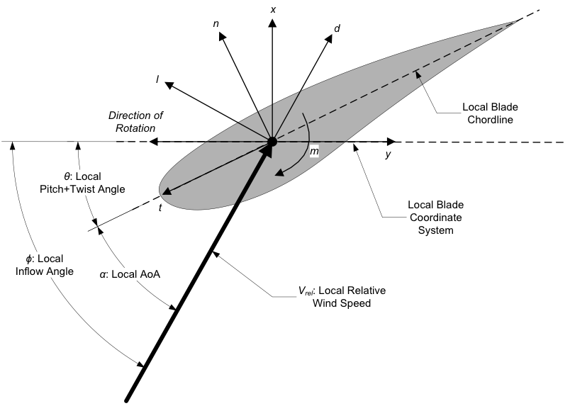
Fig. 4.4 AeroDyn Legacy Local Output Coordinate System (Looking Toward the Tip, from the Root) – l: Lift, d: Drag, m: Pitching, x: Normal (to Plane), y: Tangential (to Plane), n: Normal (to Chord), and t: Tangential (to Chord)
The \((w_{kj})\) is defined for each blade \(k\) and node \(j\), written \((w)\) for conciseness. The \((w)\) system is a transformation of the airfoil system such that this system has no rotation about the \(x\) (sweep) or \(z\) (pitch/twist) axis compared to the coned coordinate system.
The \(y_w\)-axis (in plane) of this system is orthogonal to the pitch axis, neglecting presweep and in-plane deflection.
The \(x_w\)-axis (out of plane) is normal to the deflected blade, including precurve and out-of-plane deflection.
The \(z_w\)-axis (radial) is tangent to the deflected blade, including precurve and out-of-plane deflection.
The system is constructed as follows in AeroDyn. First, the coned coordinate system \((c)\) (located at the blade root, coned, but without pitching) is defined using the following substeps and matrices:
\(\boldsymbol{R}_{bi}\): from inertial to blade root (the blade root is pitched by \(\theta_p\)).
\(\boldsymbol{R}_{hi}\): from inertial to hub.
\(\boldsymbol{R}_{bh} = \boldsymbol{R}_{bi} \boldsymbol{R}_{hi}^t=\mathop{\mathrm{Euler}}(\theta_1, \theta_2, -\theta_p)\): from hub to blade. The third Euler angle from \(\boldsymbol{R}_{bh}\) is the opposite of the pitch angle \(\theta_p\) (wind turbines use a negative convention of pitch and twist about the \(z\) axis). By setting this Euler angle to zero and constructing the transformation matrix from the two first angles, one obtains:
\(\boldsymbol{R}_{ch}=\mathop{\mathrm{Euler}}(\theta_1, \theta_2,0)\): from hub to the coned coordinate system.
\(\boldsymbol{R}_{ci}=\boldsymbol{R}_{ch} \boldsymbol{R}_{hi}\): from inertial to coned coordinate system.
Then, the \((w)\) system is defined for each airfoil cross section:
\(\boldsymbol{R}_{ai}\): from inertial to blade airfoil section (include elastic motions)
From coned system to blade airfoil section:
\[\begin{aligned} \boldsymbol{R}_{ac}=\boldsymbol{R}_{ai}\boldsymbol{R}_{ci}^t=\mathop{\mathrm{Euler}}({}^w\!\tau,{}^w\!\kappa,-{}^w\!\beta) \label{eq:R_acBetaFull} \end{aligned}\]where \({}^w\!\beta\) contains the full twist (aerodynamic, elastic and pitch), \({}^w\!\tau\) would be the toe angle (but it is not used) \({}^w\!\kappa\) is the cant angle (stored as
Curve). We use the supperscript \(w\) because these angles are defined as part of the \((w)\) system.
\(\boldsymbol{R}_{wc}=\mathop{\mathrm{Euler}}(0,{}^w\!\kappa,0)\): from coned system to \(w\)-system. The \((w)\) system keeps only the rotation about \(y_c\) (\(\approx\)prebend), thereby neglecting the ones about \(x\) (sweep) and \(z\) (\(\approx\) twist+pitch).
\(\boldsymbol{R}_{wi}=\boldsymbol{R}_{wc}\boldsymbol{R}_{ci}\): from inertial system to \(w\)-system