4.19.2. Introduction
FAST.Farm is a midfidelity multiphysics engineering tool for predicting the power performance and structural loads of wind turbines within a wind farm. FAST.Farm uses OpenFAST to solve the aero-hydro-servo-elastic dynamics of each individual turbine, but considers additional physics for wind farm-wide ambient wind in the atmospheric boundary layer; and wake deficits, advection, deflection, meandering, and merging. FAST.Farm is based on some of the principles of the dynamic wake meandering (DWM) model – including passive tracer modeling of wake meandering – but addresses many of the limitations of previous DWM implementations. FAST.Farm maintains low computational cost to support the often highly iterative and probabilistic design process. Applications of FAST.Farm include reducing wind farm underperformance and loads uncertainty, developing wind farm controls to enhance operation, optimizing wind farm siting and topology, and innovating the design of wind turbines for the wind-farm environment. The existing implementation of FAST.Farm also forms a solid foundation for further development of wind farm dynamics modeling as wind farm physics knowledge grows from future computations and experiments.
The main idea behind the DWM model is to capture key wake features pertinent to accurate prediction of wind farm power performance and wind turbine loads, including the wake-deficit evolution (important for performance) and the wake meandering and wake-added turbulence (important for loads). The wake-deficit evolution and wake meandering are illustrated in Fig. 4.55.
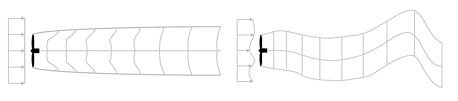
Fig. 4.55 Axisymmetric wake deficit (left) and meandering (right) evolution.
Although fundamental laws of physics are applied, appropriate simplifications have been made to minimize the computational expense, and high-fidelity modeling (HFM) solutions, e.g., using the Simulator fOr Wind Farm Applications (SOWFA), have been used to inform and calibrate the submodels. In the DWM model, the wake-flow processes are treated via the “splitting of scales,” in which small turbulent eddies (less than two diameters) affect wake-deficit evolution and large turbulent eddies (greater than two diameters) affect wake meandering.
FAST.Farm is a nonlinear time-domain multiphysics engineering tool composed of multiple submodels, each representing different physics domains of the wind farm. FAST.Farm is implemented as open-source software that follows the programming requirements of the FAST modularization framework, whereby the submodels are implemented as modules interconnected through a driver code. The submodel hierarchy of FAST.Farm is illustrated in Fig. 4.56 where the dashed lines indicated routines compiled separately from FAST.Farm.
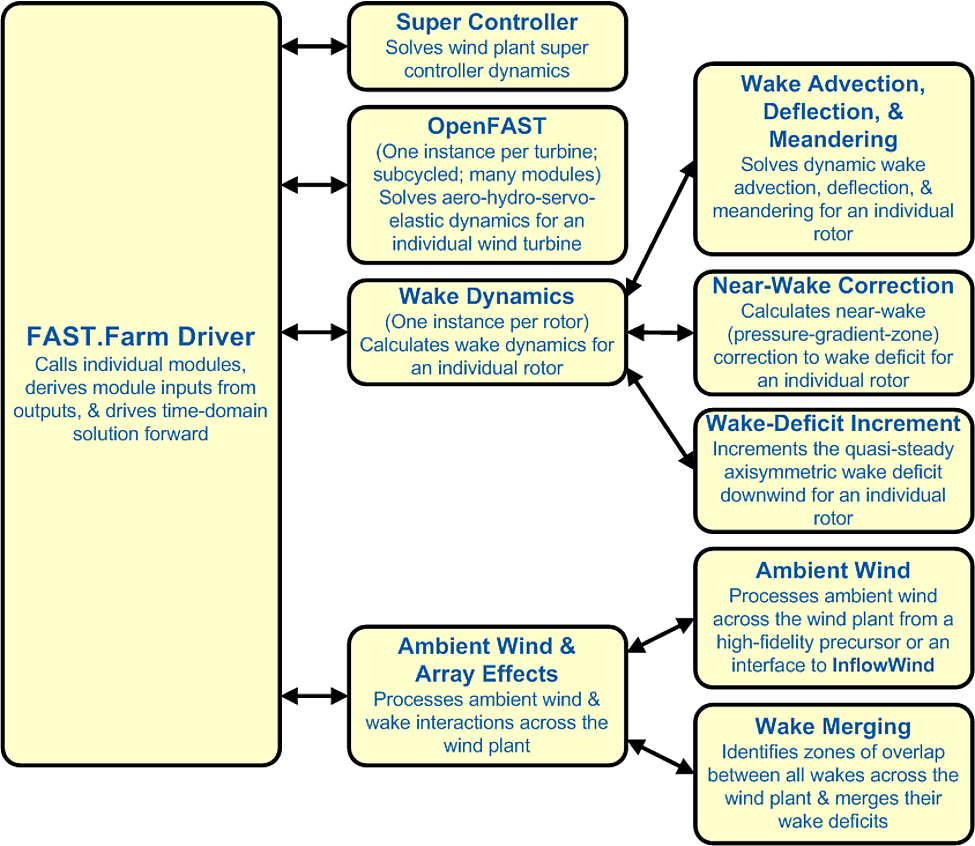
Fig. 4.56 FAST.Farm submodel hierarchy.
Wake advection, deflection, and meandering; near-wake correction; and wake-deficit increment are submodels of the wake-dynamics (WD) model, implemented in a single module. Ambient wind and wake merging are submodels of the ambient wind and array effects (AWAE) model, implemented in a single module. Combined with the OpenFAST (OF) modules, FAST.Farm has three modules and one driver. There are multiple instances of the OF and WD modules – one instance for each wind turbine/rotor.
4.19.2.1. FAST.Farm Driver
The FAST.Farm driver, also known as the “glue code,” is the code that couples individual modules together and drives the overall time-domain solution forward. Additionally, the FAST.Farm driver reads an input file of simulation parameters, checks the validity of these parameters, initializes the modules, writes results to a file, and releases memory at the end of the simulation.
4.19.2.2. OpenFAST Module
The OF module of FAST.Farm is a wrapper that enables the coupling of OpenFAST to FAST.Farm. OpenFAST models the dynamics (loads and motions) of distinct turbines in the wind farm, capturing the environmental excitations (wind inflow and, for offshore systems, waves, current, and ice) and coupled system response of the full system (the rotor, drivetrain, nacelle, tower, controller, and, for offshore systems, the substructure and station-keeping system). OpenFAST itself is an interconnection of various modules, each corresponding to different physical domains of the coupled aero-hydro-servo-elastic solution. There is one instance of the OF module for each wind turbine, which, in parallel mode, are parallelized through open multiprocessing (OpenMP). At initialization, the number of wind turbines, associated OpenFAST primary input file(s), and turbine origin(s) in the global X-Y-Z inertial-frame coordinate system are specified by the user of FAST.Farm. Turbine origins are defined as the intersection of the undeflected tower centerline and the ground or, for offshore systems, the mean sea level. The global inertial-frame coordinate system is defined with Z directed vertically upward (opposite gravity), X directed horizontally nominally downwind (along the zero-degree wind direction), and Y directed horizontally transversely. This coordinate system is not tied to specific compass directions. Among other time-dependent inputs from FAST.Farm, OpenFAST uses the disturbed wind (ambient plus wakes) across a high-resolution wind domain (in both time and space) around the turbine as input. This high-resolution domain ensures that the individual turbine loads and responses calculated by OpenFAST are accurately driven by flow through the wind farm, including wake and array effects.
4.19.2.3. Wake Dynamics Module
The WD module of FAST.Farm calculates wake dynamics for an individual rotor, including wake advection, deflection, and meandering; a near-wake correction; and a wake-deficit increment. The near-wake correction treats the near-wake (pressure-gradient zone) correction of the wake deficit. The wake-deficit increment shifts the quasi-steady-state axisymmetric wake deficit nominally downwind. There is one instance of the WD module for each rotor. The wake-dynamics calculations involve many user-specified parameters that may depend, e.g., on turbine operation or atmospheric conditions and can be calibrated to better match experimental data or by using an HFM solution as a benchmark. Default values have been derived for each calibrated parameter based on SOWFA simulations, but these can be overwritten by the user.
The wake-deficit evolution is solved in discrete time on an axisymmetric finite-difference grid consisting of a fixed number of wake planes, each with a fixed radial grid of nodes. The radial finite-difference grid can be considered a plane because the wake deficit is assumed to be axisymmetric. A wake plane can be thought of as a cross section of the wake wherein the wake deficit is calculated.
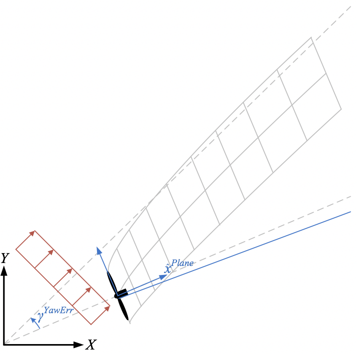
Fig. 4.57 Wake deflection resulting from inflow skew, including a horizontal wake-deflection correction. The lower dashed line represents the rotor centerline, the upper dashed line represents the wind direction, and the solid blue line represents the horizontal wake-deflection correction (offset from the rotor centerline).
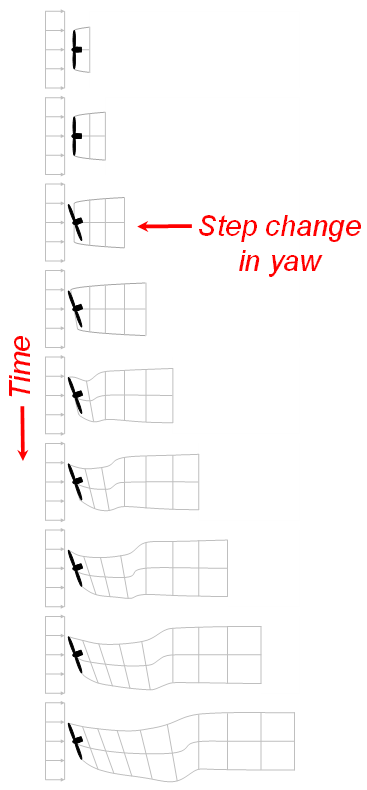
Fig. 4.58 Wake advection for a single turbine resulting from a step change in yaw angle.
By simple extensions to the passive tracer solution for transverse (horizontal and vertical) wake meandering, the wake-dynamics solution in FAST.Farm is extended to account for wake deflection, as illustrated in Fig. 4.57, and wake advection, as illustrated in Fig. 4.58, among other physical improvements such as:
Calculating the wake-plane velocities by spatially averaging the disturbed wind instead of the ambient wind (in the AWAE module)
Orientating the wake planes with the rotor centerline instead of the wind direction
Low-pass time filtering the local conditions at the rotor, as input to the wake dynamics module, to account for transients in inflow, turbine control, and/or turbine motion instead of considering time-averaged conditions.
With these extensions, the passive tracer solution enables:
The wake centerline to deflect based on inflow skew, because in skewed inflow, the wake deficit normal to the disk introduces a velocity component that is not parallel to the ambient flow
The wake to accelerate from near wake to far wake, because the wake deficits are stronger in the near wake and weaken downwind
The wake-deficit evolution to change based on conditions at the rotor, because low-pass time filtering conditions are used instead of time-averaging
The wake to meander axially in addition to transversely, because local axial winds are considered
The wake shape to be elliptical instead of circular in skewed flow when looking downwind (the wake shape remains circular when looking down the rotor centerline).
From item 1 above, a horizontally asymmetric correction to the wake deflection is accounted for, i.e., a correction to the wake deflection resulting from the wake-plane velocity, which physically results from the combination of wake rotation and shear not modeled directly in the WD module (see Fig. 4.57 for an illustration). This horizontal wake deflection correction is a simple linear correction (with a slope and offset), similar to the correction implemented in the wake model of FLORIS. Such a correction is important for accurate modeling of nacelle-yaw-based wake-redirection (wake-steering) wind farm control.
From item 3, low-pass time filtering is important because the wake reacts slowly to changes in local conditions at the rotor and because the wake evolution is treated in a quasi-steady-state fashion.
The near-wake correction submodel of the WD module computes the wake-velocity deficits at the rotor disk, as an inlet boundary condition for the wake-deficit evolution. To improve the accuracy of the far-wake solution, the near-wake correction accounts for the drop-in wind speed and radial expansion of the wake in the pressure-gradient zone behind the rotor that is not otherwise accounted for in the solution for the wake-deficit evolution.
As with most DWM implementations, the WD module of FAST.Farm models the wake-deficit evolution via the thin shear-layer approximation of the Reynolds-averaged Navier-Stokes equations under quasi-steady-state conditions in axisymmetric coordinates, with turbulence closure captured by using an eddy-viscosity formulation. The thin shear-layer approximation drops the pressure term and assumes that the velocity gradients are much bigger in the radial direction than in the axial direction.
4.19.2.4. Ambient Wind and Array Effects Module
The AWAE module of FAST.Farm processes ambient wind and wake interactions across the wind farm, including the ambient wind submodel, which processes ambient wind across the wind farm and the wake-merging submodel, which identifies zones of overlap between all wakes across the wind farm and merges their wake deficits. The calculations in the AWAE module make use of wake volumes, which are volumes formed by a (possibly curved) cylinder starting at a wake plane and extending to the next adjacent wake plane along a line connecting the centers of the two wake planes. If the adjacent wake planes (top and bottom of the cylinder) are not parallel, e.g., for transient simulations involving variations in nacelle-yaw angle, the centerline will be curved. Fig. 4.59 illustrates some of the concepts.
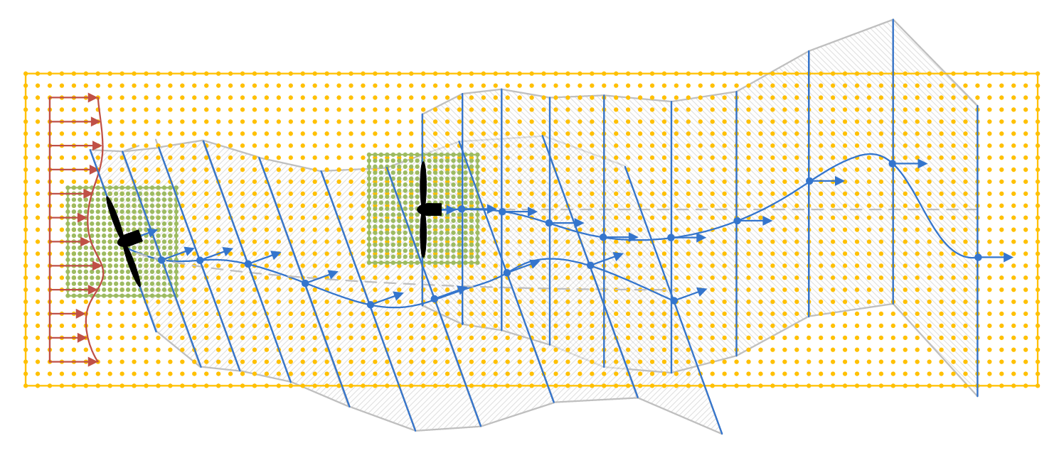
Fig. 4.59 Wake planes, wake volumes, and zones of wake overlap for a two-turbine wind farm, with the upwind turbine yawed. The yellow points represent the low-resolution wind domain and the green points represent the high-resolution wind domains around each turbine. The blue points and arrows represent the centers and orientations of the wake planes, respectively, with the wake planes identified by the blue lines normal to their orientations. The gray dashed lines represent the mean trajectory of the wake and the blue curves represent the instantaneous [meandered] trajectories. The wake volumes associated with the upwind turbine are represented by the upward hatch patterns, the wake volumes associated with the downwind turbine are represented by the downward hatch patterns, and the zones of wake overlap are represented by the crosshatch patterns. (For clarity of the illustration, the instantaneous (meandered) wake trajectory is shown as a smooth curve, but will be modeled as piece-wise linear between wake planes when adjacent wake planes are parallel. The wake planes and volumes are illustrated with a diameter equal to twice the wake diameter, but the local diameter depends on the calculation. As illustrated, a wake plane or volume may extend beyond the boundaries of the low-resolution domain of ambient wind data.)
The calculations in the AWAE module also require looping through all wind data points, turbines, and wake planes; these loops have been sped up in the parallel mode of FAST.Farm by implementation of open multiprocessing (OpenMP) parallelization.
Ambient wind may come from either a high-fidelity precursor simulation or an interface to the InflowWind module in OpenFAST. The use of the InflowWind module enables the use of simple ambient wind, e.g., uniform wind, discrete wind events, or synthetically generated turbulent wind data. Synthetically generated turbulence can be generated from, e.g., TurbSim or the Mann model, in which the wind is propagated through the wind farm using Taylor’s frozen-turbulence assumption. This method is most applicable to small wind farms or a subset of wind turbines within a larger wind farm. FAST.Farm can also use ambient wind generated by a high-fidelity precursor large-eddy simulation (LES) of the entire wind farm (without wind turbines present), such as the atmospheric boundary layer solver (ABLSolver) preprocessor of SOWFA. This atmospheric precursor simulation captures more physics than synthetic turbulence – as illustrated in Fig. 4.60 – including atmospheric stability, wind-farm-wide turbulent length scales, and complex terrain effects.
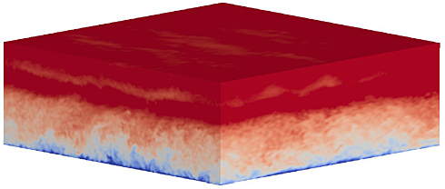
Fig. 4.60 Example flow generated by ABLSolver.
This method is more computationally expensive than using the ambient wind modeling options of InflowWind, but it is much less computationally expensive than a SOWFA simulation with wind turbines present. FAST.Farm requires ambient wind to be available in two different resolutions in both space and time. Because wind will be spatially averaged across wake planes within the AWAE module, FAST.Farm needs a low-resolution wind domain throughout the wind farm wherever turbines may potentially reside. For accurate load calculation by OpenFAST, FAST.Farm also needs high-resolution wind domains around each wind turbine (encompassing any turbine displacement). The high-resolution domains will occupy the same space as portions of the low-resolution domain, requiring domain overlap.
When using ambient wind generated by a high-fidelity precursor simulation, the AWAE module reads in the three-component wind-velocity data across the high- and low-resolution domains that were computed by the high-fidelity solver within each time step. These values are stored in files for use in a given driver time step. The wind data files, including spatial discretizations, must be in Visualization Toolkit (VTK) format and are specified by users of FAST.Farm at initialization. Visualization Toolkit is an open-source, freely available software system for three-dimensional (3D) computer graphics, image processing, and visualization. When using the InflowWind inflow option, the ambient wind across the high- and low-resolution domains are computed by calling the InflowWind module. In this case, the spatial discretizations are specified directly within the FAST.Farm primary input file. These wind data from the combined low- and high-resolution domains within a given driver time step represent the largest memory requirement of FAST.Farm.
In previous implementations of DWM, the wind turbine and wake dynamics were solved individually or serially, not considering two-way wake-merging interactions. Additionally, there was no method available to calculate the disturbed wind in zones of wake overlap. Wake merging is illustrated by the FAST.Farm simulation of Fig. 4.61.
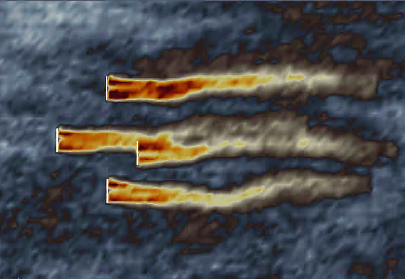
Fig. 4.61 Wake merging for closely spaced rotors.
In FAST.Farm, the wake-merging submodel of the AWAE module identifies zones of wake overlap between all wakes across the wind farm by finding wake volumes that overlap in space. Wake deficits are superimposed in the axial direction based on the root-sum-squared (RSS) method. Transverse components (radial wake deficits) are superimposed by vector sum. The RSS method assumes that the local kinetic energy of the axial deficit in a merged wake equals the sum of the local energies of the axial deficits for each wake at the given wind data point. The RSS method only applies to an array of scalars. This method works well for axial deficits because overlapping wakes likely have similar axial directions; therefore, only the magnitude of the vector is important in the superposition. A vector sum is applied to the transverse components (radial wake deficits) because any given radial direction is dependent on the azimuth angle in the axisymmetric coordinate system.
To visualize the ambient wind and wake interactions across the wind farm, FAST.Farm includes visualization capability through the generation of output files in VTK format. OpenFAST can further generate VTK-formatted output files for visualizing the wind turbine based on either surface or stick-figure geometry. The VTK files generated by FAST.Farm and OpenFAST can be read with standard open-source visualization packages such as ParaView or VisIt.
4.19.2.5. Turbine controller and super controller
FAST.Farm does not include its own modules for individual turbine controllers or farm-level controller (super controllers) but relies on separately compiled routines for them. FAST.Farm defers to the OpenFAST model of individual turbine for the turbine controller. The controller is specified in the ServoDyn module of OpenFAST. OpenFAST allows for the use of bladed-style controllers in DLL format. Tools like Reference Open Source Controller (ROSCO) can be used to design and integrate turbine controller in DLL format, if the user does not already have their own controller.
Farm-level super controller can be designed and implemented using external tools. The Hycon (Hycon) tool provides for rapid design of common farm-level controllers such as wake steering control, spatial filtering/consensus and active power control etc. Hycon includes examples demonstration the design of a wake steering controller and implementation on a small farm using FAST.Farm. The Reference Open Source Controller (ROSCO) also has wind farm control capability. It gives the user low-level access to various turbine measurements and offsets, and enables implementation of user-written, python-based controllers. ROSCO also includes examples demonstrating the implementation of a farm-level controller in FAST.Farm.
4.19.2.6. FAST.Farm Parallelization
FAST.Farm can be compiled and run in serial or parallel mode. Parallelization has been implemented in FAST.Farm through OpenMP, which allows FAST.Farm to take advantage of multicore computers by dividing computational tasks among the cores/threads within a node (but not between nodes) to speed up a single simulation. The size of the wind farm and number of wind turbines is limited only by the available random-access memory (RAM). In parallel mode, each instance of the OpenFAST submodel can be run in parallel on separate threads at the same time the ambient wind within the AWAE module is being read in another thread. Thus, the fastest simulations require at least one more core than the number of wind turbines in the wind farm. Furthermore, the output calculations within the AWAE module are parallelized into separate threads. Because of the small timescales involved and sophisticated physics, the OF submodel is the computationally slowest FAST.Farm module. The output calculation of the AWAE module is the only major calculation that cannot be solved in parallel to OpenFAST; therefore, at best, the parallelized FAST.Farm solution may execute only slightly more slowly than stand-alone OpenFAST simulations – computationally inexpensive enough to run the many simulations necessary for wind turbine/farm design and analysis.
To support the modeling of large wind farms, single simulations involving memory parallelization and parallelization between nodes of a multinode high-performance computer (HPC) through a message-passing interface (MPI) is likely required. MPI has not yet been implemented within FAST.Farm.
4.19.2.7. Organization of the Guide
The remainder of this documentation is structured as follows: Section 4.19.3 details how to obtain the FAST.Farm software archive and how to run FAST.Farm. Section 4.19.4 describes the FAST.Farm input files. Section 4.19.5 discusses the output files generated by FAST.Farm. Section 4.19.6 provides modeling guidance when using FAST.Farm. The FAST.Farm theory is covered in Section 4.19.7. Section 4.19.8 outlines future work, and the bibliography provides background and other information sources. Example FAST.Farm primary input and ambient wind data files are shown in Section 4.19.10 and Section 4.19.11. A summary of available output channels is found in Section 4.19.12.