4.2.4.1. Introduction

BeamDyn is a time-domain structural-dynamics module for slender structures created by the National Renewable Energy Laboratory (NREL) through support from the U.S. Department of Energy Wind and Water Power Program and the NREL Laboratory Directed Research and Development (LDRD) program through the grant “High-Fidelity Computational Modeling of Wind-Turbine Structural Dynamics”, see References [WJSJ15, WS13, WSJJ14, WYS13]. The module has been coupled into the FAST aero-hydro-servo-elastic wind turbine multi-physics engineering tool where it used to model blade structural dynamics. The BeamDyn module follows the requirements of the FAST modularization framework, see References [Jon13]; [GSJ13, JJ13, SJJ14], couples to FAST version 8, and provides new capabilities for modeling initially curved and twisted composite wind turbine blades undergoing large deformation. BeamDyn can also be driven as a stand-alone code to compute the static and dynamic responses of slender structures (blades or otherwise) under prescribed boundary and applied loading conditions uncoupled from FAST.

The model underlying BeamDyn is the geometrically exact beam theory (GEBT) [Hod06]. GEBT supports full geometric nonlinearity and large deflection, with bending, torsion, shear, and extensional degree-of-freedom (DOFs); anisotropic composite material couplings (using full \(6 \times 6\) mass and stiffness matrices, including bend-twist coupling); and a reference axis that permits blades that are not straight (supporting built-in curve, sweep, and sectional offsets). The GEBT beam equations are discretized in space with Legendre spectral finite elements (LSFEs). LFSEs are p-type elements that combine the accuracy of global spectral methods with the geometric modeling flexibility of the h-type finite elements (FEs) [Pat84]. For smooth solutions, LSFEs have exponential convergence rates compared to low-order elements that have algebraic convergence [SG03, WS13] . Two spatial numerical integration schemes are implemented for the finite element inner products: reduced Gauss quadrature and trapezoidal-rule integration. Trapezoidal-rule integration is appropriate when a large number of sectional properties are specified along the beam axis, for example, in a long wind turbine blade with material properties that vary dramatically over the length. Time integration of the BeamDyn equations of motion is achieved through the implicit generalized- \(\alpha\) solver, with user-specified numerical damping. The combined GEBT-LSFE approach permits users to model a long, flexible, composite wind turbine blade with a single high-order element. Given the theoretical foundation and powerful numerical tools introduced above, BeamDyn can solve the complicated nonlinear composite beam problem in an efficient manner. For example, it was recently shown that a grid-independent dynamic solution of a 50-m composite wind turbine blade and with dozens of cross-section stations could be achieved with a single \(7^{th}\)-order LSFE [WSJJ16].

When coupled with FAST, loads and responses are transferred between BeamDyn, ElastoDyn, ServoDyn, and AeroDyn via the FAST driver program (glue code) to enable aero-elasto-servo interaction at each coupling time step. There is a separate instance of BeamDyn for each blade. At the root node, the inputs to BeamDyn are the six displacements (three translations and three rotations), six velocities, and six accelerations; the root node outputs from BeamDyn are the six reaction loads (three translational forces and three moments). BeamDyn also outputs the blade displacements, velocities, and accelerations along the beam length, which are used by AeroDyn to calculate the local aerodynamic loads (distributed along the length) that are used as inputs for BeamDyn. In addition, BeamDyn can calculate member internal reaction loads, as requested by the user. Please refers to Figure [fig:FlowChart] for the coupled interactions between BeamDyn and other modules in FAST. When coupled to FAST, BeamDyn replaces the more simplified blade structural model of ElastoDyn that is still available as an option, but is only applicable to straight isotropic blades dominated by bending. When uncoupled from FAST, the root motion (boundary condition) and applied loads are specified via a stand-alone BeamDyn driver code.

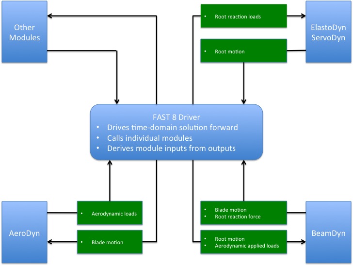
Fig. 4.27 Coupled interaction between BeamDyn and FAST

The BeamDyn input file defines the blade geometry; cross-sectional material mass, stiffness, and damping properties; FE resolution; and other simulation- and output-control parameters. The blade geometry is defined through a curvilinear blade reference axis by a series of key points in three-dimensional (3D) space along with the initial twist angles at these points. Each member contains at least three key points for the cubic spline fit implemented in BeamDyn; each member is discretized with a single LSFE with a parameter defining the order of the element. Note that the number of key points defining the member and the order (\(N\)) of the LSFE are independent. LSFE nodes, which are located at the \(N+1\) Gauss-Legendre-Lobatto points, are not evenly spaced along the element; node locations are generated by the module based on the mesh information. Blade properties are specified in a non-dimensional coordinate ranging from 0.0 to 1.0 along the blade reference axis and are linearly interpolated between two stations if needed by the spatial integration method. The BeamDyn applied loads can be either distributed loads specified at quadrature points, concentrated loads specified at FE nodes, or a combination of the two. When BeamDyn is coupled to FAST, the blade analysis node discretization may be independent between BeamDyn and AeroDyn.

This document is organized as follows. Section Running BeamDyn details how to obtain the BeamDyn and FAST software archives and run either the stand-alone version of BeamDyn or BeamDyn coupled to FAST. Section Input Files describes the BeamDyn input files. Section Output Files discusses the output files generated by BeamDyn. Section BeamDyn Theory summarizes the BeamDyn theory. Section Future Work outlines potential future work. Example input files are shown in Appendix Section 4.2.4.8.1. A summary of available output channels is found in Appendix BeamDyn List of Output Channels.