4.7.3. Input Files
Users specify the blade model parameters; including its geometry, cross-sectional properties, and FE and output control parameters; via a primary BeamDyn input file and a blade property input file. When used in stand-alone mode, an additional driver input file is required. This driver file specifies inputs normally provided to BeamDyn by FAST, including simulation range, root motions, and externally applied loads.
No lines should be added or removed from the input files, except in tables where the number of rows is specified.
4.7.3.1. Units
BeamDyn uses the SI system (kg, m, s, N). Angles are assumed to be in radians unless otherwise specified.
4.7.3.2. BeamDyn Driver Input File
The driver input file is needed only for the stand-alone version of BeamDyn. It contains inputs that are normally set by FAST and that are necessary to control the simulation for uncoupled models.
The driver input file begins with two lines of header information, which is for the user but is not used by the software. If BeamDyn is run in the stand-alone mode, the results output file will be prefixed with the same name of this driver input file.
A sample BeamDyn driver input file is given in Section 4.7.8.1.
4.7.3.2.1. Simulation Control Parameters
DynamicSolve is a logical variable that specifies if BeamDyn should use dynamic analysis (DynamicSolve = true)
or static analysis (DynamicSolve = false).
t_initial and t_final specify the starting time of the simulation and ending time of the simulation, respectively.
dt specifies the time step size.
4.7.3.2.2. Gravity Parameters
Gx , Gy , and Gz specify the components of gravity vector along \(X\), \(Y\), and \(Z\) directions in the global coordinate system, respectively.
In FAST, this is normally 0, 0, and -9.80665.
4.7.3.2.3. Inertial Frame Parameters
This section defines the relation between two inertial frames, the global coordinate system and initial blade reference coordinate system.
GlbPos(1), GlbPos(2), and GlbPos(3) specify three components of the initial global position vector along \(X\), \(Y\), and \(Z\) directions resolved in the global coordinate system, see Figure Fig. 4.29.
And the following \(3 \times 3\) direction cosine matrix (GlbDCM) relates the rotations from the global coordinate system to the initial blade reference coordinate system.
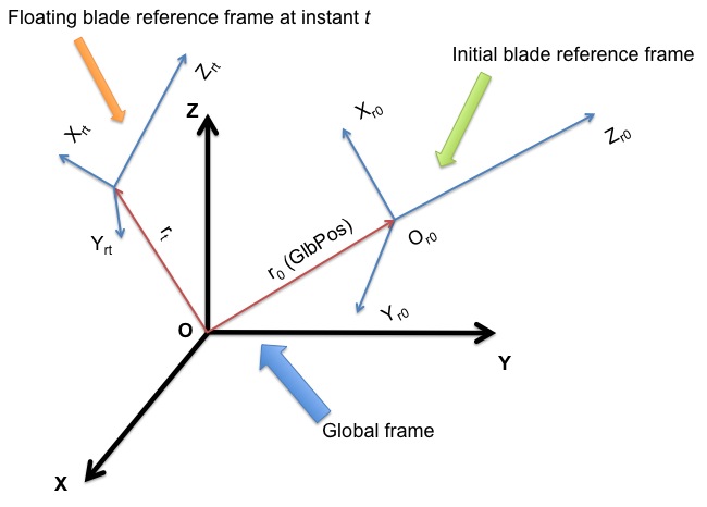
Fig. 4.29 Global and blade coordinate systems in BeamDyn.
4.7.3.2.4. Blade Floating Reference Frame Parameters
This section specifies the parameters that define the blade floating reference frame, which is a body-attached floating frame; the blade root is cantilevered at the origin of this frame. Based on the driver input file, the floating blade reference fame is assumed to be in a constant rigid-body rotation mode about the origin of the global coordinate system, that is,
where \(v_{rt}\) is the root (origin of the floating blade reference frame) translational velocity vector; \(\omega_r\) is the constant root (origin of the floating blade reference frame) angular velocity vector; and \(r_t\) is the global position vector introduced in the previous section at instant \(t\), see Fig. 4.29.
The floating blade reference frame coincides with the initial floating blade reference frame at the beginning \(t=0\).
RootVel(4), RootVel(5), and RootVel(6) specify the three components of the constant root angular velocity vector about \(X\), \(Y\), and \(Z\) axises in global coordinate system, respectively.
RootVel(1), RootVel(2), and RootVel(3), which are the three components of the root translational velocity vector along \(X\), \(Y\), and \(Z\) directions in global coordinate system, respectively, are calculated based on Eq. (4.69).
BeamDyn can handle more complicated root motions by changing, for example, the BD_InputSolve subroutine in the Driver_Beam.f90
(requiring a recompile of stand-alone BeamDyn).
The blade is initialized in the rigid-body motion mode, i.e., based on the root velocity information defined in this section and the position information defined in the previous section, the motion of other points along the blade are initialized as
where \(a_{0}\) is the initial translational acceleration vector along the blade; \(v_0\) and \(\omega_0\) the initial translational and angular velocity vectors along the blade, respectively; and \(P\) is the position vector along the blade relative to the root. Note that these equations are actually implemented with a call to the NWTC Library’s mesh mapping routines.
4.7.3.2.5. Applied Load
This section defines the applied loads, including distributed, point (lumped), and tip-concentrated loads, for the stand-alone analysis.
The first six entries DistrLoad(i), \(i \in [1,6]\), specify three
components of uniformly distributed force vector and three components of
uniformly distributed moment vector in the global coordinate systems,
respectively.
The following six entries TipLoad(i),
\(i \in [1,6]\), specify three components of concentrated tip force
vector and three components of concentrated tip moment vector in the
global coordinate system, respectively.
NumPointLoads defines how many point loads along the blade will be applied. The table
following this input contains two header lines with seven columns and NumPointLoads rows.
The first column is the non-dimensional distance along the local blade reference axis,
ranging from \([0.0,1.0]\). The next three columns, Fx, Fy, and Fz specify three
components of point-force vector. The remaining three columns, Mx, My, and Mz specify three
components of a moment vector.
The distributed load defined in this section is assumed to be uniform along the blade and constant throughout the simulation. The tip load is a constant concentrated load applied at the tip of a blade.
It is noted that all the loads defined in this section are dead loads, i.e., they are not rotating with the blade following the rigid-body rotation defined in the previous section.
BeamDyn is capable of handling more complex loading cases, e.g.,
time-dependent loads, through customization of the source code
(requiring a recompile of stand-alone BeamDyn). The user can define such
loads in the BD_InputSolve subroutine in the Driver_Beam.f90 file,
which is called every time step. The following section can be modified
to define the concentrated load at each FE node:
u%PointLoad%Force(1:3,u%PointLoad%NNodes)  = u%PointLoad%Force(1:3,u%PointLoad%NNodes)  + DvrData%TipLoad(1:3)
u%PointLoad%Moment(1:3,u%PointLoad%NNodes) = u%PointLoad%Moment(1:3,u%PointLoad%NNodes) + DvrData%TipLoad(4:6)
where the first index in each array ranges from 1 to 3 for load vector
components along three global directions and the second index of each
array ranges from 1 to u%PointLoad%NNodes, where the latter is the total
number of FE nodes. Note that u%PointLoad%Force(1:3,:) and u%PointLoad%Moment(1:3,:)
have been populated with the point-load loads read from the BeamDyn driver input file
using the call to Transfer_Point_to_Point earlier in the subroutine.
For example, a time-dependent sinusoidal force acting along the \(X\) direction applied at the \(2^{nd}\) FE node can be defined as
u%PointLoad%Force(:,:) = 0.0D0
u%PointLoad%Force(1,2)  = 1.0D+03*SIN((2.0*pi)*t/6.0 )
u%PointLoad%Moment(:,:) = 0.0D0
with 1.0D+03 being the amplitude and 6.0 being the
period. Note that this particular implementation overrides the tip-load and point-loads
defined in the driver input file.
Similar to the concentrated load, the distributed loads can be defined in the same subroutine
DO i=1,u%DistrLoad%NNodes
   u%DistrLoad%Force(1:3,i) = DvrData%DistrLoad(1:3)
   u%DistrLoad%Moment(1:3,i)= DvrData%DistrLoad(4:6)
ENDDO
where u%DistrLoad%NNodes is the number of nodes input to BeamDyn (on the quadrature points),
and DvrData%DistrLoad(:) is the constant uniformly distributed load BeamDyn reads from the driver
input file. The user can modify DvrData%DistrLoad(:) to define the loads based on need.
We note that the distributed loads are defined at the quadrature points
for numerical integrations. For example, if Gauss quadrature is chosen,
then the distributed loads are defined at
Gauss points plus the two end points of the beam (root and tip). For
trapezoidal quadrature, p%ngp stores the number of trapezoidal
quadrature points.
4.7.3.2.6. Primary Input File
InputFile is the file name of the primary BeamDyn input file. This
name should be in quotations and can contain an absolute path or a
relative path.
4.7.3.3. BeamDyn Primary Input File
The BeamDyn primary input file defines the blade geometry, LSFE-discretization and simulation options, output channels, and name of the blade input file. The geometry of the blade is defined by key-point coordinates and initial twist angles (in units of degree) in the blade local coordinate system (IEC standard blade system where \(Z_r\) is along blade axis from root to tip, \(X_r\) directs normally toward the suction side, and \(Y_r\) directs normally toward the trailing edge).
The file is organized into several functional sections. Each section corresponds to an aspect of the BeamDyn model.
A sample BeamDyn primary input file is given in Section 4.7.8.
The primary input file begins with two lines of header information, which are for the user but are not used by the software.
4.7.3.3.1. Simulation Controls
The user can set the Echo flag to TRUE to have BeamDyn echo the
contents of the BeamDyn input file (useful for debugging errors in the
input file).
The QuasiStaticInit flag indicates if BeamDyn should perform a quasi-static
solution at initialization to better initialize its states. This option is only
available when coupled to OpenFAST with dynamic analysis enabled. When set to TRUE,
BeamDyn will perform a steady-state startup (SSS) solve that includes centripetal
accelerations to reduce startup transients and improve numerical performance. This
is particularly useful for rotating blade simulations where the initial conditions
would otherwise cause spurious transients. The keyword “DEFAULT” sets this to FALSE.
rhoinf specifies the numerical damping parameter (spectral radius
of the amplification matrix) in the range of \([0.0,1.0]\) used in
the generalized-\(\alpha\) time integrator implemented in BeamDyn
for dynamic analysis. Note: This parameter is only used when BeamDyn is run
in loose coupling mode (e.g., stand-alone with the driver or when loose coupling
is explicitly selected in OpenFAST). When tight coupling is used in OpenFAST,
time integration is handled by the glue code and this parameter is ignored.
For rhoinf = 1.0, no numerical damping is introduced and the
generalized-\(\alpha\) scheme is identical to the Newmark scheme; for
rhoinf = 0.0, maximum numerical damping is
introduced. Numerical damping may help produce numerically stable
solutions.
Quadrature specifies the spatial numerical integration scheme.
There are two options: 1) Gauss quadrature; and 2) Trapezoidal
quadrature. We note that in the current version, Gauss quadrature is
implemented in reduced form to improve efficiency and avoid shear
locking. In the trapezoidal quadrature, only one member (FE element) can
be defined in the following GEOMETRY section of the primary input file.
Trapezoidal quadrature is appropriate when the number of “blade input
stations” (described below) is significantly greater than the order of
the LSFE.
Refine specifies a refinement parameter used in trapezoidal
quadrature. An integer value greater than unity will split the space
between two input stations into “Refine factor” of segments. The keyword
“DEFAULT” may be used to set it to 1, i.e., no refinement is needed.
This entry is not used in Gauss quadrature.
N_Fact specifies a parameter used in the modified Newton-Raphson
scheme. Note: This parameter is only used when BeamDyn is run in loose coupling
mode (stand-alone with the driver or when loose coupling is explicitly selected in
OpenFAST). When tight coupling is used in OpenFAST, this parameter is ignored.
If N_Fact = 1 a full Newton iteration scheme is used, i.e., the global tangent
stiffness matrix is computed and factorized at each iteration; if
N_Fact > 1 a modified Newton iteration
scheme is used, i.e., the global stiffness matrix is computed and
factorized every N_Fact iterations within each time step. The
keyword “DEFAULT” sets N_Fact = 5.
DTBeam specifies the constant time increment of the
time-integration in seconds. The keyword “DEFAULT” may be used to
indicate that the module should employ the time increment prescribed by
the driver code (FAST/stand-alone driver program).
load_retries specifies the maximum number of load retries allowed. This option
currently works only for static analysis. For every load retry, the applied load is
halved to promote convergence of the Newton-Raphson scheme in iteration of smaller
load steps as opposed to one single large load step which may cause divergence of the
Newton-Raphson scheme. The keyword “DEFAULT” sets load_retries = 20.
NRMax specifies the maximum number of iterations per time step in
the Newton-Raphson scheme. Note: This parameter is only used when BeamDyn is run
in loose coupling mode (stand-alone with the driver or when loose coupling is explicitly
selected in OpenFAST). When tight coupling is used in OpenFAST, this parameter is ignored.
If convergence is not reached within this number of iterations, BeamDyn returns an error
message and terminates the simulation. The keyword “DEFAULT” sets
NRMax = 10.
Stop_Tol specifies a tolerance parameter used in convergence
criteria of a nonlinear solution that is used for the termination of the
iteration. Note: This parameter is only used when BeamDyn is run in loose coupling
mode (stand-alone with the driver or when loose coupling is explicitly selected in
OpenFAST). When tight coupling is used in OpenFAST, this parameter is ignored.
The keyword “DEFAULT” sets Stop_Tol = 1.0E-05. Please refer to
Section 4.7.5.7 for more details.
tngt_stf_fd is a boolean that sets the flag to compute the tangent stiffness
matrix using finite differencing instead of analytical differentiation. The
finite differencing is performed using a central scheme. The keyword “DEFAULT”
sets tngt_stf_fd = FALSE.
tngt_stf_comp is a boolean that sets the flag to compare the analytical tangent
stiffness matrix against the finite differenced tangent stiffness matrix. Information is
written to the terminal regarding the dof where the maximum difference is observed. If
tngt_stf_fd = FALSE and tngt_stf_comp = TRUE, the analytical tangent stiffness
matrix is used to solve the system of equations while the finite difference tangent stiffness
matrix is used only to perform the comparison of the two matrices. The keyword “DEFAULT”
sets tngt_stf_comp = FALSE.
tngt_stf_pert sets the perturbation size for finite differencing. The “DEFAULT” value
based on experience is set to 1e-06.
tngt_stf_difftol is the maximum allowable relative difference between the analytical
and finite differenced tangent stiffness matrices. If for any entry in the matrices,
the relative difference exceeds this value the simulation will terminate. The “DEFAULT” value
is currently set to 1e-01.
RotStates is a flag that indicates if BeamDyn’s continuous states should be
oriented in the rotating frame during linearization analysis when coupled to OpenFAST.
If multi-blade coordinate (MBC3) analysis is performed, RotStates must be true.
4.7.3.3.2. Geometry Parameter
The blade geometry is defined by a curvilinear local blade reference axis. The blade reference axis locates the origin and orientation of each a local coordinate system where the cross-sectional 6x6 stiffness and mass matrices are defined in the BeamDyn blade input file. It should not really matter where in the cross section the 6x6 stiffness and mass matrices are defined relative to, as long as the reference axis is consistently defined and closely follows the natural geometry of the blade.
The blade beam model is composed of several members in contiguous series and each member is defined by at least three key points in BeamDyn. A cubic-spline-fit pre-processor implemented in BeamDyn automatically generates the member based on the key points and then interconnects the members into a blade. There is always a shared key point at adjacent members; therefore the total number of key points is related to number of members and key points in each member.
member_total specifies the total number of beam members used in
the structure. With the LSFE discretization, a single member and a
sufficiently high element order, order_elem below, may well be
sufficient.
kp_total specifies the total number of key points used to define
the beam members.
The following section contains member_total lines. Each line has
two integers providing the member number (must be 1, 2, 3, etc.,
sequentially) and the number of key points in this member, respectively.
It is noted that the number of key points in each member is not
independent of the total number of key points and they should satisfy
the following equality:
where \(n_i\) is the number of key points in the \(i^{th}\) member. Because cubic splines are implemented in BeamDyn, \(n_i\) must be greater than or equal to three. Figures Fig. 4.30 and Fig. 4.31 show two cases for member and key-point definition.
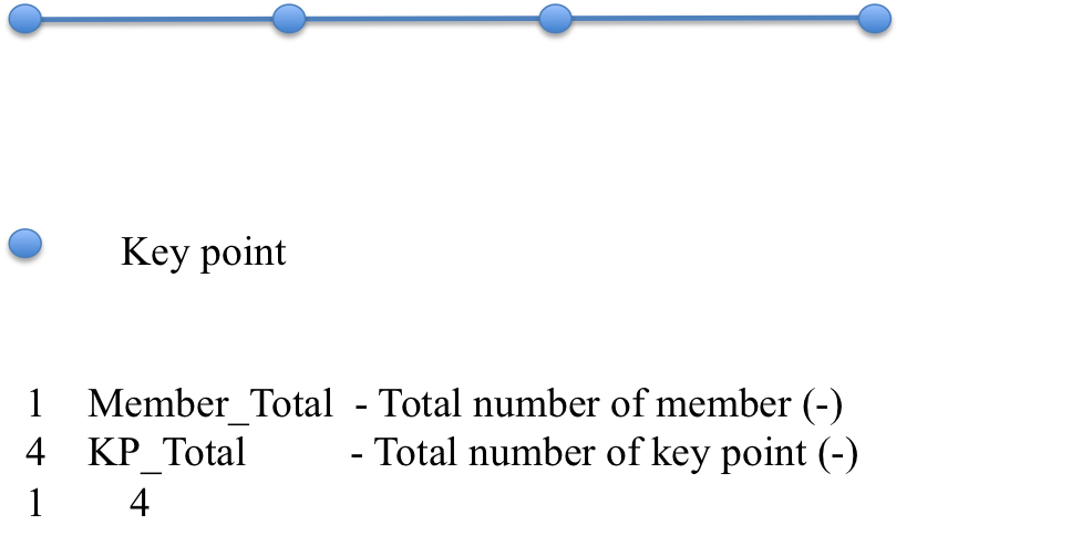
Fig. 4.30 Member and key point definition: one member defined by four key points;
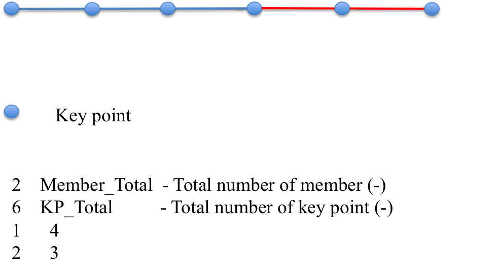
Fig. 4.31 Member and key point definition: two members defined by six key points.
The next section defines the key-point information, preceded by two
header lines. Each key point is defined by three physical coordinates
(kp_xr, kp_yr, kp_zr) in the IEC standard blade
coordinate system (the blade reference coordinate system) along with a
structural twist angle (initial_twist) in the unit of degrees.
The structural twist angle is also following the IEC standard which is
defined as the twist about the negative \(Z_l\) axis. The key points
are entered sequentially (from the root to tip) and there should be a
total of kp_total lines for BeamDyn to read in the information,
after two header lines. Please refer to Fig. 4.32 for
more details on the blade geometry definition.
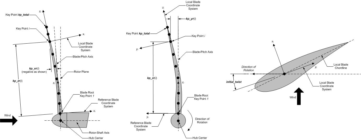
Fig. 4.32 BeamDyn Blade Geometry - Top: Side View; Middle: Front View (Looking Downwind); Bottom: Cross Section View (Looking Toward the Tip, from the Root)
4.7.3.3.3. Mesh Parameter
Order_Elem specifies the order of shape functions for each finite
element. Each LSFE will have Order_Elem+1 nodes located at the
GLL quadrature points. All LSFEs will have the same order. With the LSFE
discretization, an increase in accuracy will, in general, be better
achieved by increasing Order_Elem (i.e., \(p\)-refinement)
rather than increasing the number of members (i.e.,
\(h\)-refinement). For Gauss quadrature, Order_Elem should be
greater than one.
4.7.3.3.4. Material Parameter
BldFile is the file name of the blade input file. This name should
be in quotations and can contain an absolute path or a relative path.
4.7.3.3.5. Outputs
In this section of the primary input file, the user sets flags and switches for the desired output behavior.
Specifying SumPrint = TRUE causes BeamDyn to generate a
summary file with name InputFile.sum. See
Section 4.7.4.2 for summary file details.
OutFmt parameter controls the formatting of the results within the
stand-alone BeamDyn output file. It needs to be a valid Fortran format
string, but BeamDyn currently does not check the validity. This input is
unused when BeamDyn is used coupled to FAST.
NNodeOuts specifies the number of nodes where output can be
written to a file. Currently, BeamDyn can output quantities at a maximum
of nine nodes.
OutNd is a list NNodeOuts long of node numbers between 1 and the number of
nodes on the output mesh, separated by any
combination of commas, semicolons, spaces, and/or tabs. The nodal
positions are given in the summary file, if output.
For Gassian quadrature, the number of nodes on the output mesh is the total number of FE nodes;
for trapezoidal quadrature, this is the number of quadrature nodes.
The OutList block contains a list of output parameters. Enter one
or more lines containing quoted strings that in turn contain one or more
output parameter names. Separate output parameter names by any
combination of commas, semicolons, spaces, and/or tabs. If you prefix a
parameter name with a minus sign, “-“, underscore, “_”, or the
characters “m” or “M”, BeamDyn will multiply the value for that channel
by -1 before writing the data. The parameters are written in the order
they are listed in the input file. BeamDyn allows you to use multiple
lines so that you can break your list into meaningful groups and so the
lines can be shorter. You may enter comments after the closing quote on
any of the lines. Entering a line with the string “END” at the beginning
of the line or at the beginning of a quoted string found at the
beginning of the line will cause BeamDyn to quit scanning for more lines
of channel names. Node-related quantities are generated for the
requested nodes identified through the OutNd list above. If BeamDyn
encounters an unknown/invalid channel name, it warns the users but will
remove the suspect channel from the output file. Please refer to
Appendix Section 4.7.8.2 for a complete list of possible output
parameters and their names.
4.7.3.3.6. Nodal Outputs
In addition to the named outputs in Section 4.7.3.3.5 above, BeamDyn allows
for outputting the full set blade node motions and loads (tower nodes
unavailable at present). Please refer to the BeamDyn_Nodes tab in the
Excel file OutListParameters.xlsx
for a complete list of possible output parameters.
This section follows the END statement from normal Outputs section described above, and includes a separator description line followed by the following optinos.
BldNd_BlOutNd specifies which nodes to output. This is currently unused.
The OutList section controls the nodal output quantities generated by BeamDyn. In this section, the user specifies the name of the channel family to output. The output name for each channel is then created internally by BeamDyn by combining the blade number, node number, and channel family name. For example, if the user specifies TDxr as the channel family name, the output channels will be named with the convention of B\(\mathbf{\beta}\)N###TDxr where \(\mathbf{\beta}\) is the blade number, and ### is the three digit node number.
4.7.3.3.6.1. Sample Nodal Outputs section
This sample includes the END statement from the regular outputs section.
  1END of input file (the word "END" must appear in the first 3 columns of this last OutList line)
  2---------------------- NODE OUTPUTS --------------------------------------------
  3         99   BldNd_BlOutNd   - Blade nodes on each blade (currently unused)
  4              OutList     - The next line(s) contains a list of output parameters.  See OutListParameters.xlsx, BeamDyn_Nodes tab for a listing of available output channels, (-)
  5"FxL"       - Sectional force resultants at each node expressed in l    l: a floating coordinate system local to the deflected beam    (N)
  6"FyL"       - Sectional force resultants at each node expressed in l    l: a floating coordinate system local to the deflected beam    (N)
  7"FzL"       - Sectional force resultants at each node expressed in l    l: a floating coordinate system local to the deflected beam    (N)
  8"MxL"       - Sectional moment resultants at each node expressed in l    l: a floating coordinate system local to the deflected beam    (N-m)
  9"MyL"       - Sectional moment resultants at each node expressed in l    l: a floating coordinate system local to the deflected beam    (N-m)
 10"MzL"       - Sectional moment resultants at each node expressed in l    l: a floating coordinate system local to the deflected beam    (N-m)
 11"Fxr"       - Sectional force resultants at each node expressed in r    r: a floating reference coordinate system fixed to the root of the moving beam; when coupled to FAST for blades, this is equivalent to the IEC blade (b) coordinate system    (N)
 12"Fyr"       - Sectional force resultants at each node expressed in r    r: a floating reference coordinate system fixed to the root of the moving beam; when coupled to FAST for blades, this is equivalent to the IEC blade (b) coordinate system    (N)
 13"Fzr"       - Sectional force resultants at each node expressed in r    r: a floating reference coordinate system fixed to the root of the moving beam; when coupled to FAST for blades, this is equivalent to the IEC blade (b) coordinate system    (N)
 14"Mxr"       - Sectional moment resultants at each node expressed in r    r: a floating reference coordinate system fixed to the root of the moving beam; when coupled to FAST for blades, this is equivalent to the IEC blade (b) coordinate system    (N-m)
 15"Myr"       - Sectional moment resultants at each node expressed in r    r: a floating reference coordinate system fixed to the root of the moving beam; when coupled to FAST for blades, this is equivalent to the IEC blade (b) coordinate system    (N-m)
 16"Mzr"       - Sectional moment resultants at each node expressed in r    r: a floating reference coordinate system fixed to the root of the moving beam; when coupled to FAST for blades, this is equivalent to the IEC blade (b) coordinate system    (N-m)
 17"TDxr"      - Sectional translational deflection (relative to the undeflected position) at each node expressed in r    r: a floating reference coordinate system fixed to the root of the moving beam; when coupled to FAST for blades, this is equivalent to the IEC blade (b) coordinate system    (m)
 18"TDyr"      - Sectional translational deflection (relative to the undeflected position) at each node expressed in r    r: a floating reference coordinate system fixed to the root of the moving beam; when coupled to FAST for blades, this is equivalent to the IEC blade (b) coordinate system    (m)
 19"TDzr"      - Sectional translational deflection (relative to the undeflected position) at each node expressed in r    r: a floating reference coordinate system fixed to the root of the moving beam; when coupled to FAST for blades, this is equivalent to the IEC blade (b) coordinate system    (m)
 20"RDxr"      - Sectional angular/rotational deflection Wiener-Milenkovic parameter (relative to the undeflected orientation) at each node expressed in r    r: a floating reference coordinate system fixed to the root of the moving beam; when coupled to FAST for blades, this is equivalent to the IEC blade (b) coordinate system    (-)
 21"RDyr"      - Sectional angular/rotational deflection Wiener-Milenkovic parameter (relative to the undeflected orientation) at each node expressed in r    r: a floating reference coordinate system fixed to the root of the moving beam; when coupled to FAST for blades, this is equivalent to the IEC blade (b) coordinate system    (-)
 22"RDzr"      - Sectional angular/rotational deflection Wiener-Milenkovic parameter (relative to the undeflected orientation) at each node expressed in r    r: a floating reference coordinate system fixed to the root of the moving beam; when coupled to FAST for blades, this is equivalent to the IEC blade (b) coordinate system    (-)
 23"AbsXg"     - Node position in X (global coordinate)     g: the global inertial frame coordinate system; when coupled to FAST, this is equivalent to FAST’s global inertial frame (i) coordinate system     (m)
 24"AbsYg"     - Node position in Y (global coordinate)     g: the global inertial frame coordinate system; when coupled to FAST, this is equivalent to FAST’s global inertial frame (i) coordinate system     (m)
 25"AbsZg"     - Node position in Z (global coordinate)     g: the global inertial frame coordinate system; when coupled to FAST, this is equivalent to FAST’s global inertial frame (i) coordinate system     (m)
 26"AbsXr"     - Node position in X (relative to root)     r: a floating reference coordinate system fixed to the root of the moving beam; when coupled to FAST for blades, this is equivalent to the IEC blade (b) coordinate system     (m)
 27"AbsYr"     - Node position in Y (relative to root)     r: a floating reference coordinate system fixed to the root of the moving beam; when coupled to FAST for blades, this is equivalent to the IEC blade (b) coordinate system     (m)
 28"AbsZr"     - Node position in Z (relative to root)     r: a floating reference coordinate system fixed to the root of the moving beam; when coupled to FAST for blades, this is equivalent to the IEC blade (b) coordinate system     (m)
 29"TVxg"      - Sectional translational velocities (absolute)    g: the global inertial frame coordinate system; when coupled to FAST, this is equivalent to FAST’s global inertial frame (i) coordinate system     (m/s)
 30"TVyg"      - Sectional translational velocities (absolute)    g: the global inertial frame coordinate system; when coupled to FAST, this is equivalent to FAST’s global inertial frame (i) coordinate system     (m/s)
 31"TVzg"      - Sectional translational velocities (absolute)    g: the global inertial frame coordinate system; when coupled to FAST, this is equivalent to FAST’s global inertial frame (i) coordinate system     (m/s)
 32"TVxl"      - Sectional translational velocities (absolute)    l: a floating coordinate system local to the deflected beam    (m/s)
 33"TVyl"      - Sectional translational velocities (absolute)    l: a floating coordinate system local to the deflected beam    (m/s)
 34"TVzl"      - Sectional translational velocities (absolute)    l: a floating coordinate system local to the deflected beam    (m/s)
 35"TVxr"      - Sectional translational velocities (absolute)    r: a floating reference coordinate system fixed to the root of the moving beam; when coupled to FAST for blades, this is equivalent to the IEC blade (b) coordinate system     (m/s)
 36"TVyr"      - Sectional translational velocities (absolute)    r: a floating reference coordinate system fixed to the root of the moving beam; when coupled to FAST for blades, this is equivalent to the IEC blade (b) coordinate system     (m/s)
 37"TVzr"      - Sectional translational velocities (absolute)    r: a floating reference coordinate system fixed to the root of the moving beam; when coupled to FAST for blades, this is equivalent to the IEC blade (b) coordinate system     (m/s)
 38"RVxg"      - Sectional angular/rotational velocities (absolute)    g: the global inertial frame coordinate system; when coupled to FAST, this is equivalent to FAST’s global inertial frame (i) coordinate system     (deg/s)
 39"RVyg"      - Sectional angular/rotational velocities (absolute)    g: the global inertial frame coordinate system; when coupled to FAST, this is equivalent to FAST’s global inertial frame (i) coordinate system     (deg/s)
 40"RVzg"      - Sectional angular/rotational velocities (absolute)    g: the global inertial frame coordinate system; when coupled to FAST, this is equivalent to FAST’s global inertial frame (i) coordinate system     (deg/s)
 41"RVxl"      - Sectional angular/rotational velocities (absolute)    l: a floating coordinate system local to the deflected beam    (deg/s)
 42"RVyl"      - Sectional angular/rotational velocities (absolute)    l: a floating coordinate system local to the deflected beam    (deg/s)
 43"RVzl"      - Sectional angular/rotational velocities (absolute)    l: a floating coordinate system local to the deflected beam    (deg/s)
 44"RVxr"      - Sectional angular/rotational velocities (absolute)    r: a floating reference coordinate system fixed to the root of the moving beam; when coupled to FAST for blades, this is equivalent to the IEC blade (b) coordinate system     (deg/s)
 45"RVyr"      - Sectional angular/rotational velocities (absolute)    r: a floating reference coordinate system fixed to the root of the moving beam; when coupled to FAST for blades, this is equivalent to the IEC blade (b) coordinate system     (deg/s)
 46"RVzr"      - Sectional angular/rotational velocities (absolute)    r: a floating reference coordinate system fixed to the root of the moving beam; when coupled to FAST for blades, this is equivalent to the IEC blade (b) coordinate system     (deg/s)
 47"TAxl"      - Sectional angular/rotational velocities (absolute)    l: a floating coordinate system local to the deflected beam    (m/s^2)
 48"TAyl"      - Sectional angular/rotational velocities (absolute)    l: a floating coordinate system local to the deflected beam    (m/s^2)
 49"TAzl"      - Sectional angular/rotational velocities (absolute)    l: a floating coordinate system local to the deflected beam    (m/s^2)
 50"TAxr"      - Sectional angular/rotational velocities (absolute)    r: a floating reference coordinate system fixed to the root of the moving beam; when coupled to FAST for blades, this is equivalent to the IEC blade (b) coordinate system     (m/s^2)
 51"TAyr"      - Sectional angular/rotational velocities (absolute)    r: a floating reference coordinate system fixed to the root of the moving beam; when coupled to FAST for blades, this is equivalent to the IEC blade (b) coordinate system     (m/s^2)
 52"TAzr"      - Sectional angular/rotational velocities (absolute)    r: a floating reference coordinate system fixed to the root of the moving beam; when coupled to FAST for blades, this is equivalent to the IEC blade (b) coordinate system     (m/s^2)
 53"RAxl"      - Sectional angular/rotational velocities (absolute)    l: a floating coordinate system local to the deflected beam    (deg/s^2)
 54"RAyl"      - Sectional angular/rotational velocities (absolute)    l: a floating coordinate system local to the deflected beam    (deg/s^2)
 55"RAzl"      - Sectional angular/rotational velocities (absolute)    l: a floating coordinate system local to the deflected beam    (deg/s^2)
 56"RAxr"      - Sectional angular/rotational velocities (absolute)    r: a floating reference coordinate system fixed to the root of the moving beam; when coupled to FAST for blades, this is equivalent to the IEC blade (b) coordinate system     (deg/s^2)
 57"RAyr"      - Sectional angular/rotational velocities (absolute)    r: a floating reference coordinate system fixed to the root of the moving beam; when coupled to FAST for blades, this is equivalent to the IEC blade (b) coordinate system     (deg/s^2)
 58"RAzr"      - Sectional angular/rotational velocities (absolute)    r: a floating reference coordinate system fixed to the root of the moving beam; when coupled to FAST for blades, this is equivalent to the IEC blade (b) coordinate system     (deg/s^2)
 59"PFxL"      - Applied point forces at each node expressed in l    l: a floating coordinate system local to the deflected beam    (N)
 60"PFyL"      - Applied point forces at each node expressed in l    l: a floating coordinate system local to the deflected beam    (N)
 61"PFzL"      - Applied point forces at each node expressed in l    l: a floating coordinate system local to the deflected beam    (N)
 62"PMxL"      - Applied point moments at each node expressed in l    l: a floating coordinate system local to the deflected beam    (N-m)
 63"PMyL"      - Applied point moments at each node expressed in l    l: a floating coordinate system local to the deflected beam    (N-m)
 64"PMzL"      - Applied point moments at each node expressed in l    l: a floating coordinate system local to the deflected beam    (N-m)
 65"DFxL"      - Applied distributed forces at each node expressed in l    l: a floating coordinate system local to the deflected beam    (N/m)
 66"DFyL"      - Applied distributed forces at each node expressed in l    l: a floating coordinate system local to the deflected beam    (N/m)
 67"DFzL"      - Applied distributed forces at each node expressed in l    l: a floating coordinate system local to the deflected beam    (N/m)
 68"DMxL"      - Applied distributed moments at each node expressed in l    l: a floating coordinate system local to the deflected beam    (N-m/m)
 69"DMyL"      - Applied distributed moments at each node expressed in l    l: a floating coordinate system local to the deflected beam    (N-m/m)
 70"DMzL"      - Applied distributed moments at each node expressed in l    l: a floating coordinate system local to the deflected beam    (N-m/m)
 71"DFxR"      - Applied distributed forces at each node expressed in r    r: a floating reference coordinate system fixed to the root of the moving beam; when coupled to FAST for blades, this is equivalent to the IEC blade (b) coordinate system     (N/m)
 72"DFyR"      - Applied distributed forces at each node expressed in r    r: a floating reference coordinate system fixed to the root of the moving beam; when coupled to FAST for blades, this is equivalent to the IEC blade (b) coordinate system     (N/m)
 73"DFzR"      - Applied distributed forces at each node expressed in r    r: a floating reference coordinate system fixed to the root of the moving beam; when coupled to FAST for blades, this is equivalent to the IEC blade (b) coordinate system     (N/m)
 74"DMxR"      - Applied distributed forces at each node expressed in r    r: a floating reference coordinate system fixed to the root of the moving beam; when coupled to FAST for blades, this is equivalent to the IEC blade (b) coordinate system     (N-m/m)
 75"DMyR"      - Applied distributed forces at each node expressed in r    r: a floating reference coordinate system fixed to the root of the moving beam; when coupled to FAST for blades, this is equivalent to the IEC blade (b) coordinate system     (N-m/m)
 76"DMzR"      - Applied distributed forces at each node expressed in r    r: a floating reference coordinate system fixed to the root of the moving beam; when coupled to FAST for blades, this is equivalent to the IEC blade (b) coordinate system     (N-m/m)
 77"FFbxl"     - Gyroscopic force x     l: a floating coordinate system local to the deflected beam    (N)
 78"FFbyl"     - Gyroscopic force y     l: a floating coordinate system local to the deflected beam    (N)
 79"FFbzl"     - Gyroscopic force z     l: a floating coordinate system local to the deflected beam    (N)
 80"FFbxr"     - Gyroscopic force x     r: a floating reference coordinate system fixed to the root of the moving beam; when coupled to FAST for blades, this is equivalent to the IEC blade (b) coordinate system     (N)
 81"FFbyr"     - Gyroscopic force y     r: a floating reference coordinate system fixed to the root of the moving beam; when coupled to FAST for blades, this is equivalent to the IEC blade (b) coordinate system     (N)
 82"FFbzr"     - Gyroscopic force z     r: a floating reference coordinate system fixed to the root of the moving beam; when coupled to FAST for blades, this is equivalent to the IEC blade (b) coordinate system     (N)
 83"MFbxl"     - Gyroscopic moment about x     l: a floating coordinate system local to the deflected beam    (N-m)
 84"MFbyl"     - Gyroscopic moment about y     l: a floating coordinate system local to the deflected beam    (N-m)
 85"MFbzl"     - Gyroscopic moment about z     l: a floating coordinate system local to the deflected beam    (N-m)
 86"MFbxr"     - Gyroscopic moment about x     r: a floating reference coordinate system fixed to the root of the moving beam; when coupled to FAST for blades, this is equivalent to the IEC blade (b) coordinate system     (N-m)
 87"MFbyr"     - Gyroscopic moment about y     r: a floating reference coordinate system fixed to the root of the moving beam; when coupled to FAST for blades, this is equivalent to the IEC blade (b) coordinate system     (N-m)
 88"MFbzr"     - Gyroscopic moment about z     r: a floating reference coordinate system fixed to the root of the moving beam; when coupled to FAST for blades, this is equivalent to the IEC blade (b) coordinate system     (N-m)
 89"FFcxl"     - Elastic restoring force Fc x     l: a floating coordinate system local to the deflected beam    (N)
 90"FFcyl"     - Elastic restoring force Fc y     l: a floating coordinate system local to the deflected beam    (N)
 91"FFczl"     - Elastic restoring force Fc z     l: a floating coordinate system local to the deflected beam    (N)
 92"FFcxr"     - Elastic restoring force Fc x     r: a floating reference coordinate system fixed to the root of the moving beam; when coupled to FAST for blades, this is equivalent to the IEC blade (b) coordinate system     (N)
 93"FFcyr"     - Elastic restoring force Fc y     r: a floating reference coordinate system fixed to the root of the moving beam; when coupled to FAST for blades, this is equivalent to the IEC blade (b) coordinate system     (N)
 94"FFczr"     - Elastic restoring force Fc z     r: a floating reference coordinate system fixed to the root of the moving beam; when coupled to FAST for blades, this is equivalent to the IEC blade (b) coordinate system     (N)
 95"MFcxl"     - Elastic restoring moment Fc about x     l: a floating coordinate system local to the deflected beam    (N-m)
 96"MFcyl"     - Elastic restoring moment Fc about y     l: a floating coordinate system local to the deflected beam    (N-m)
 97"MFczl"     - Elastic restoring moment Fc about z     l: a floating coordinate system local to the deflected beam    (N-m)
 98"MFcxr"     - Elastic restoring moment Fc about x     r: a floating reference coordinate system fixed to the root of the moving beam; when coupled to FAST for blades, this is equivalent to the IEC blade (b) coordinate system     (N-m)
 99"MFcyr"     - Elastic restoring moment Fc about y     r: a floating reference coordinate system fixed to the root of the moving beam; when coupled to FAST for blades, this is equivalent to the IEC blade (b) coordinate system     (N-m)
100"MFczr"     - Elastic restoring moment Fc about z     r: a floating reference coordinate system fixed to the root of the moving beam; when coupled to FAST for blades, this is equivalent to the IEC blade (b) coordinate system     (N-m)
101"FFdxl"     - Elastic restoring force Fd x     l: a floating coordinate system local to the deflected beam    (N)
102"FFdyl"     - Elastic restoring force Fd y     l: a floating coordinate system local to the deflected beam    (N)
103"FFdzl"     - Elastic restoring force Fd z     l: a floating coordinate system local to the deflected beam    (N)
104"FFdxr"     - Elastic restoring force Fd x     r: a floating reference coordinate system fixed to the root of the moving beam; when coupled to FAST for blades, this is equivalent to the IEC blade (b) coordinate system     (N)
105"FFdyr"     - Elastic restoring force Fd y     r: a floating reference coordinate system fixed to the root of the moving beam; when coupled to FAST for blades, this is equivalent to the IEC blade (b) coordinate system     (N)
106"FFdzr"     - Elastic restoring force Fd z     r: a floating reference coordinate system fixed to the root of the moving beam; when coupled to FAST for blades, this is equivalent to the IEC blade (b) coordinate system     (N)
107"MFdxl"     - Elastic restoring moment Fd about x     l: a floating coordinate system local to the deflected beam    (N-m)
108"MFdyl"     - Elastic restoring moment Fd about y     l: a floating coordinate system local to the deflected beam    (N-m)
109"MFdzl"     - Elastic restoring moment Fd about z     l: a floating coordinate system local to the deflected beam    (N-m)
110"MFdxr"     - Elastic restoring moment Fd about x     r: a floating reference coordinate system fixed to the root of the moving beam; when coupled to FAST for blades, this is equivalent to the IEC blade (b) coordinate system     (N-m)
111"MFdyr"     - Elastic restoring moment Fd about y     r: a floating reference coordinate system fixed to the root of the moving beam; when coupled to FAST for blades, this is equivalent to the IEC blade (b) coordinate system     (N-m)
112"MFdzr"     - Elastic restoring moment Fd about z     r: a floating reference coordinate system fixed to the root of the moving beam; when coupled to FAST for blades, this is equivalent to the IEC blade (b) coordinate system     (N-m)
113"FFgxl"     - Gravity force x     l: a floating coordinate system local to the deflected beam    (N)
114"FFgyl"     - Gravity force y     l: a floating coordinate system local to the deflected beam    (N)
115"FFgzl"     - Gravity force z     l: a floating coordinate system local to the deflected beam    (N)
116"FFgxr"     - Gravity force x     r: a floating reference coordinate system fixed to the root of the moving beam; when coupled to FAST for blades, this is equivalent to the IEC blade (b) coordinate system     (N)
117"FFgyr"     - Gravity force y     r: a floating reference coordinate system fixed to the root of the moving beam; when coupled to FAST for blades, this is equivalent to the IEC blade (b) coordinate system     (N)
118"FFgzr"     - Gravity force z     r: a floating reference coordinate system fixed to the root of the moving beam; when coupled to FAST for blades, this is equivalent to the IEC blade (b) coordinate system     (N)
119"MFgxl"     - Gravity moment about x     l: a floating coordinate system local to the deflected beam    (N-m)
120"MFgyl"     - Gravity moment about y     l: a floating coordinate system local to the deflected beam    (N-m)
121"MFgzl"     - Gravity moment about z     l: a floating coordinate system local to the deflected beam    (N-m)
122"MFgxr"     - Gravity moment about x     r: a floating reference coordinate system fixed to the root of the moving beam; when coupled to FAST for blades, this is equivalent to the IEC blade (b) coordinate system     (N-m)
123"MFgyr"     - Gravity moment about y     r: a floating reference coordinate system fixed to the root of the moving beam; when coupled to FAST for blades, this is equivalent to the IEC blade (b) coordinate system     (N-m)
124"MFgzr"     - Gravity moment about z     r: a floating reference coordinate system fixed to the root of the moving beam; when coupled to FAST for blades, this is equivalent to the IEC blade (b) coordinate system     (N-m)
125"FFixl"     - Inertial force x     l: a floating coordinate system local to the deflected beam    (N)
126"FFiyl"     - Inertial force y     l: a floating coordinate system local to the deflected beam    (N)
127"FFizl"     - Inertial force z     l: a floating coordinate system local to the deflected beam    (N)
128"FFixr"     - Inertial force x     r: a floating reference coordinate system fixed to the root of the moving beam; when coupled to FAST for blades, this is equivalent to the IEC blade (b) coordinate system     (N)
129"FFiyr"     - Inertial force y     r: a floating reference coordinate system fixed to the root of the moving beam; when coupled to FAST for blades, this is equivalent to the IEC blade (b) coordinate system     (N)
130"FFizr"     - Inertial force z     r: a floating reference coordinate system fixed to the root of the moving beam; when coupled to FAST for blades, this is equivalent to the IEC blade (b) coordinate system     (N)
131"MFixl"     - Inertial moment about x     l: a floating coordinate system local to the deflected beam    (N-m)
132"MFiyl"     - Inertial moment about y     l: a floating coordinate system local to the deflected beam    (N-m)
133"MFizl"     - Inertial moment about z     l: a floating coordinate system local to the deflected beam    (N-m)
134"MFixr"     - Inertial moment about x     r: a floating reference coordinate system fixed to the root of the moving beam; when coupled to FAST for blades, this is equivalent to the IEC blade (b) coordinate system     (N-m)
135"MFiyr"     - Inertial moment about y     r: a floating reference coordinate system fixed to the root of the moving beam; when coupled to FAST for blades, this is equivalent to the IEC blade (b) coordinate system     (N-m)
136"MFizr"     - Inertial moment about z     r: a floating reference coordinate system fixed to the root of the moving beam; when coupled to FAST for blades, this is equivalent to the IEC blade (b) coordinate system     (N-m)
137END of input file (the word "END" must appear in the first 3 columns of this last OutList line)
138---------------------------------------------------------------------------------------
4.7.3.4. Blade Input File
The blade input file defines the cross-sectional properties at various stations along a blade and six damping coefficient for the whole blade. A sample BeamDyn blade input file is given in Section 4.7.8. The blade input file begins with two lines of header information, which is for the user but is not used by the software.
4.7.3.4.1. Blade Parameters
Station_Total specifies the number cross-sectional stations along
the blade axis used in the analysis.
damp_type specifies the type of structural damping to be used in the
analysis. There are three options:
damp_type = 0: No damping is considered in the analysis. The damping coefficients in the following sections will be ignored.damp_type = 1: Stiffness-proportional damping is applied. The six damping coefficients (beta) in the Stiffness-Proportional Damping section are used to scale the 6x6 stiffness matrix at each cross section.damp_type = 2: Modal damping is applied. The modal fractions of critical damping (zeta) for the firstn_modesmodes are used. BeamDyn internally computes the modal properties and applies damping in the modal coordinates.
4.7.3.4.2. Stiffness-Proportional Damping Coefficients
This section specifies six damping coefficients, \(\mu_{ii}\) (also called beta) with
\(i \in [1,6]\), for six DOFs (three translations and three
rotations). These coefficients are only used when damp_flag = 1.
Viscous damping is implemented in BeamDyn where the damping forces are proportional to the strain rate. These are stiffness-proportional damping coefficients, whereby the \(6\times6\) damping matrix at each cross section is scaled from the \(6 \times 6\) stiffness matrix by these diagonal entries of a \(6 \times 6\) scaling matrix:
where \(\mathcal{\underline{F}}^{Damp}\) is the damping force, \(\underline{\underline{S}}\) is the \(6 \times 6\) cross-sectional stiffness matrix, \(\dot{\underline{\epsilon}}\) is the strain rate, and \(\underline{\underline{\mu}}\) is the damping coefficient matrix defined as
4.7.3.4.3. Modal Damping Coefficients
This section specifies modal damping parameters and is only used when damp_flag = 2.
n_modes specifies the number of modes for which modal damping coefficients
are provided. BeamDyn will compute the natural frequencies and mode shapes of the
blade and apply damping in the modal coordinates.
zeta is an array of n_modes modal damping ratios, one for each mode.
Each value should typically be between 0.0 (no damping) and 1.0 (critical damping),
though higher values are permitted. Common values for composite blade structures
are less than 0.05 (less than 5% of critical damping). The damping
ratios are applied to modes 1 through n_modes in order of increasing frequency.
After n_modes damping values are assigned that grow proportional to the modal
natural frequency. This proportionality is assigned to match the zeta value
of last mode with prescribed damping.
If modal damping is selected, BeamDyn calculates nodal damping forces based on the node velocities, rotated to the initial node orientation, and the mode shape after quasi-static initialization has been performed, if it was requested. These nodal damping forces are then transformed back to the current node orientation.
When using modal damping, PitchDOF needs to be set to TRUE in ElastoDyn to give BeamDyn
a correct root pitch velocity. Otherwise, blade pitching will give spurious damping behavior.
Recommendations:
It is recommended to stop inputting zeta values before reaching the first axial mode (typically around 18 modes). Users may experiment with including more or fewer modes to observe the effect on results.
Avoid prescribing a final zeta value of 1.0 (e.g., do not specify 18 modes with realistic zeta values followed by a 19th mode with zeta=1.0), as this can significantly degrade result quality.
When attempting to match stiffness-proportional damping (\(\mu\)), the OpenFAST toolbox may fail to provide reliable damping values matched with mode numbers once some modes become critically damped. Reducing the number of modes (e.g., from 40 to 30) can help if higher modes are indexed incorrectly.
In some cases, axial loads appear to be driven by the axial motion of non-axial modes.
Verify that the modal frequencies and modal participation factors output in
InputFile.BD.R*.B*.modes.csvfile are consistent with the expected modes. This file is only output when modal damping is used. The number of output modes in this file is equal to the degrees of freedom of the blade. However, modes tend to become numerical artifacts past the first few modes of a given type.
Notes:
Modal damping is experimental in OpenFAST 5.0, so should be used with care.
Modal damping is mainly supported for tight coupling with OpenFAST.
In some cases, when used with loose coupling or BeamDyn Driver, a much smaller time step may be needed to get reaction forces to converge with the tight coupling case and/or stiffness-proportional damping (\(\mu\)) case.
Output forces internal forces from BeamDyn at quadrature points do not capture contributions from the modal damping forces.
4.7.3.4.4. Distributed Properties
This section specifies the cross-sectional properties at each of the
Station_Total stations. For each station, a non-dimensional
parameter \(\eta\) specifies the station location along the local
blade reference axis ranging from \([0.0,1.0]\). The first and last
station parameters must be set to \(0.0\) (for the blade root) and
\(1.0\) (for the blade tip), respectively.
Following the station location parameter \(\eta\), there are two \(6 \times 6\) matrices providing the structural and inertial properties for this cross-section. First is the stiffness matrix and then the mass matrix. We note that these matrices are defined in a local coordinate system along the blade axis with \(Z_{l}\) directing toward the unit tangent vector of the blade reference axis. For a cross-section without coupling effects, for example, the stiffness matrix is given as follows:
where \(K_{ShrEdg}\) and \(K_{ShrFlp}\) are the edge and flap shear stiffnesses, respectively; \(EA\) is the extension stiffness; \(EI_{Edg}\) and \(EI_{Flp}\) are the edge and flap stiffnesses, respectively; and \(GJ\) is the torsional stiffness. It is pointed out that for a generic cross-section, the sectional property matrices can be derived from a sectional analysis tool, e.g. VABS, BECAS, or NuMAD/BPE.
A generalized sectional mass matrix is given by:
where \(m\) is the mass density per unit span; \(X_{cm}\) and \(Y_{cm}\) are the local coordinates of the sectional center of mass, respectively; \(i_{Edg}\) and \(i_{Flp}\) are the edge and flap mass moments of inertia per unit span, respectively; \(i_{plr}\) is the polar moment of inertia per unit span; and \(i_{cp}\) is the sectional cross-product of inertia per unit span. We note that for beam structure, the \(i_{plr}\) is given as (although this relationship is not checked by BeamDyn)