4.2.3.5. Model Verification

4.2.3.5.1. Reference Wind Turbine

The noise model of OpenFAST is exercised by simulating the aeroacoustics noise emissions of the IEA Wind Task 37 land-based reference wind turbine ([aa-BTD+19]). The main characteristics of the reference wind turbine are presented in Table 4.2.

Table 4.2 Main Characteristics of the IEA Wind Task 37 Land-Based Reference Wind Turbine

Data	Value	Data	Value
Wind class	International Electrotechnical Commision 3A	Rated electrical power	3.37 megawatts
Rated aerodynamic power	3.6 megawatts	Drivetrain & generator efficiency	93.60%
Rotor diameter	130 meters	Hub height	110 meters
Cut-in wind speed	4 meters/second	Cut-out wind speed	25 meters/second
Rotor cone angle	3 degrees	Nacelle tilt angle	5 degrees
Max blade tip speed	80 meters/second	Rated tip-speed ratio	8.16
Maximum aerodynamic Cp	0.481	Rated rotor speed	11.75 revolutions per minute

The OpenFAST model of the wind turbine is available at https://github.com/OpenFAST/r-test and is optionally coupled to the Reference OpenSource Controller. 2

4.2.3.5.2. Code-to-Code Comparison

A detailed code-to-code comparison was conducted to verify the implementation of the noise models linked to OpenFAST with the implementation available at the Wind Energy Institute of the Technical University of Munich, Germany. The latter is described in Sucameli ([aa-SBCB18]) and is implemented in the wind turbine design framework Cp-Max, which adopts the multibody-based aeroservoelastic solver Cp-Lambda.

The comparison is conducted for the main noise sources—turbulent inflow and the TBL-TE noise—for both the single airfoil profile and full turbine. This helped resolve a few implementation mistakes and small inconsistencies. The comparison is performed with a steady wind of 8 meters per second (m/s), no shear, a rated pitch angle of 1.17 degrees (deg), and a fixed rotor speed of 10.04 revolutions per minute (rpm). A fixed value of 0.1 is assumed for the incident turbulent intensity, \(I_{1}\).

Fig. 4.17 shows the predictions in terms of SPL for the Amiet model with the angle-of-attack correction from OpenFAST, the Simplified Guidati model generated by OpenFAST, and the Amiet model from Cp-Max.

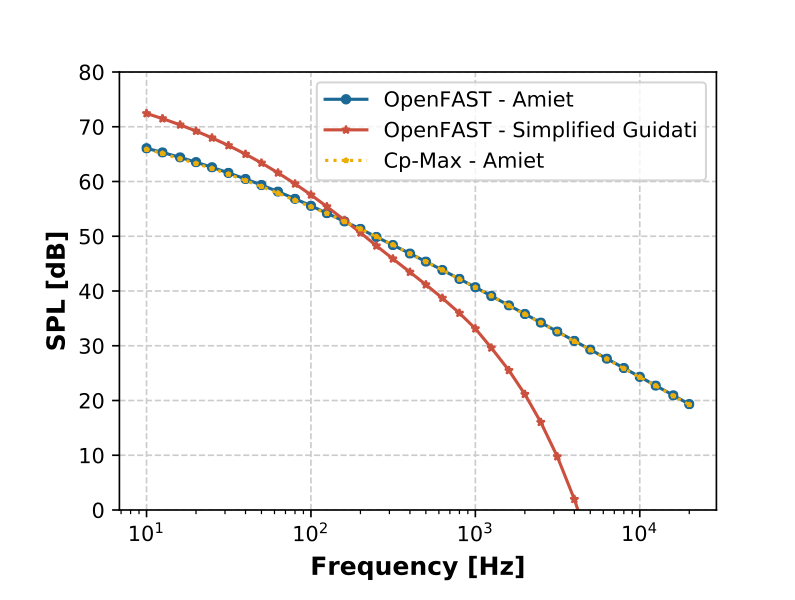
Fig. 4.17 Code-to-code comparison for the TI models

The two implementations of the turbulent inflow Amiet model return a perfect match between OpenFAST and Cp-Max. The chosen scenario sees the blade operating at optimal angles of attack and, therefore, the effect of the angle of attack correction is negligible. The plots also show the great difference between the Amiet model and the Simplified Guidati model. It may be useful to keep in mind that the Simplified Guidati model has, in the past, been corrected with a factor of +10 dB, which is applied here.

For the same inflow and rotor conditions, the BPM and TNO TBL-TE noise models are compared in Fig. 4.18. The match is again satisfactory, although slightly larger differences emerge that are attributed to differences in the angles of attack between the two aeroelastic solvers and in different integration schemes in the TNO formulations.

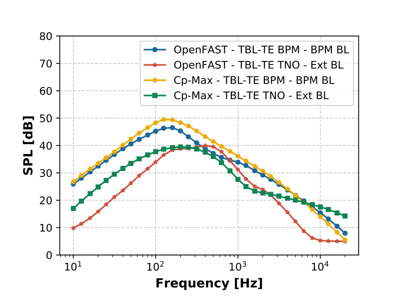
Fig. 4.18 Code-to-code comparison for the BPM and TNO TBL-TE models. The boundary layer properties are estimated from either the BPM model (BPM BL) or defined by the user (Ext BL)

The last comparison looked at the directivity models and the overall sound pressure levels at various observer locations. Simulations are run distributing 200 observers in a horizontal square of 500 meters (m) by 500 m (see Fig. 4.19). The noise is computed from the Amiet and the BPM turbulent boundary layer-trailing edge models. The code-to-code comparison returns similar predictions between OpenFAST and Cp-Max. The comparison is shown in Fig. 4.20.

The main conclusion of this code-to-code comparison is that, to the best of authors’ knowledge, the models are now implemented correctly and generate similar SPL and overall SPL levels for any arbitrary observer. Nonetheless, it is clear that all of the presented models are imperfect, and improvements could be made both at the theoretical implementation levels.

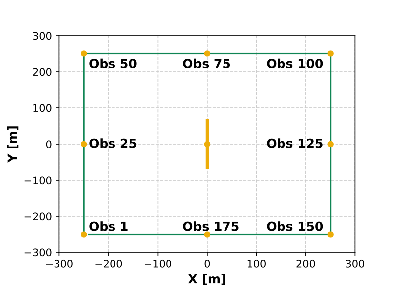
Fig. 4.19 Location and numbering of the observers

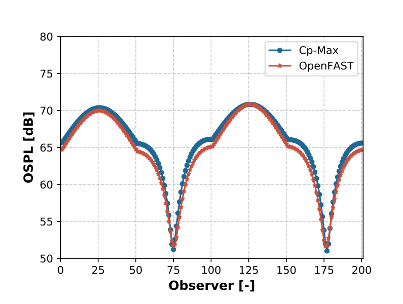
Fig. 4.20 Comparison of overall sound pressure levels for the observers distributed, as shown in the previous figure

4.2.3.5.3. Model Usage

The aeroacoustics model of OpenFAST has four options for the outputs:

1. Overall sound pressure level (dB/A-weighted decibels [dBA])—one value per time step per observer is generated

2. Total sound pressure level spectra (dB/dBA)—one spectrum per time step per observer is generated between 10 Hz and 20 kHz

3. Mechanism-dependent sound pressure level spectra (dB/dBA)—one spectrum per active noise mechanism per time step per observer is generated between 10 Hz and 20 kHz.

4. Overall sound pressure level (dB/A-weighted decibels [dBA])—one value per blade per node per time step per observer is generated

The overall SPL from the first option can be used to plot directivity maps of the noise. An example, which was generated using a Python script, 3 is shown in Fig. 4.21. The noise map, which shows the overall SPL averaged over 1 rotor revolution, is generated for a steady wind speed of 8 m/s, a fixed rotor speed of 10.04 rpm, and a 1.17-deg pitch angle. In a horizontal circle of 500 m in diameter, 1681 observers are placed at a 2-m height. Only the Simplified Guidati and the BPM TBL-TE noise models are activated.

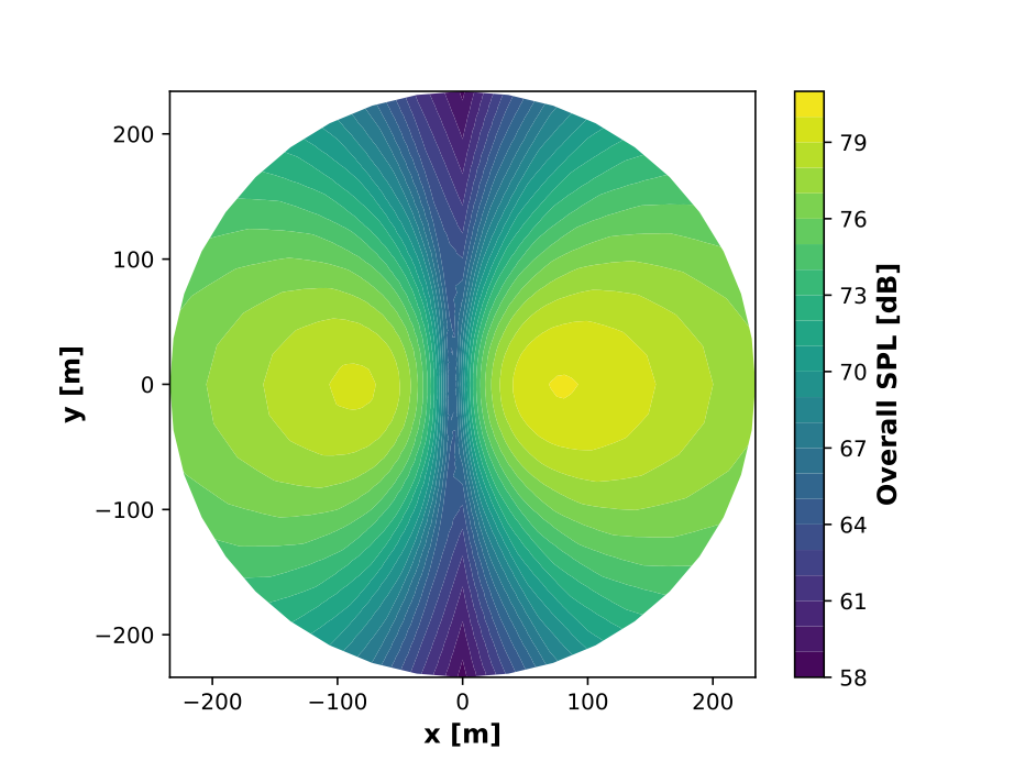
Fig. 4.21 Map of the overall SPL of the reference wind turbine at a 2-m height from Simplified Guidati and BPM TBL-TE noise models. The wind turbine is located at x=0, y=0. A steady wind of 8 m/s blows from left (-x) to right (+x).

The second output can be used to generate SPL spectra. These spectra can be computed for various observers and optionally A-weighted to account for human hearing. Fig. 4.22 shows the total SPL spectra computed for the same rotor conditions of the previous example. The A-weight greatly reduces the curve at frequency below 1,000 Hz while slightly increasing those between 1 kHz and 8 kHz.

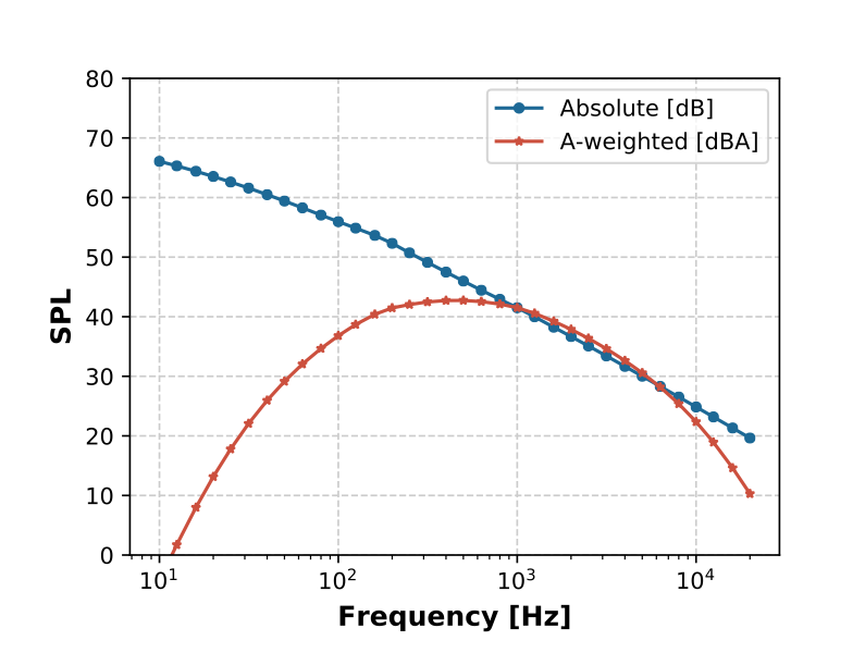
Fig. 4.22 Comparison between absolute and A-weighted SPL

The third output distinguishes the SPL spectrum per mechanism. Fig. 4.23 shows the various SPL spectra estimated by each noise model for the same rotor conditions reported earlier. The total spectrum is visibly dominated by the turbulent inflow, TBL-TE, and trailing-edge bluntness noise mechanisms. Notably, the latter is extremely sensitive to its inputs, \(\Psi\) and \(h\). The reference wind turbine is a purely numerical model, and these quantities have been arbitrarily set. Users should pay attention to these inputs when calling the trailing-edge bluntness model. Consistent with literature, the laminar boundary layer-vortex shedding and tip vortex noise mechanisms have negative dB values and are, therefore, not visible. Notably, these spectra are not A-weighted, but users can activate the flag and obtain A-weighted spectra.

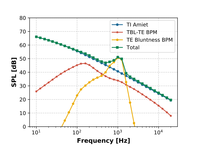
Fig. 4.23 Nonweighted SPL spectra of the various noise mechanisms

Finally, the fourth output can be used to visualize the noise emission across the rotor. Fig. 4.24 shows the noise generation of the rotor as seen from an observer located 175 meters downwind at a height of 2 meters. The map is generated by plotting the overall SPL generated by one blade during one rotor revolution. The plot shows that higher noise is observed when the blade is descending (the rotor from behind is seen rotating counterclockwise). This effect, which matches the results shown in [aa-MM03], is explained by the asymmetry of (4.60). Noise is indeed higher when the observer faces the leading edge of an airfoil (high \(\Theta_e\)), than when it faces the trailing edge (low \(\Theta_e\)).

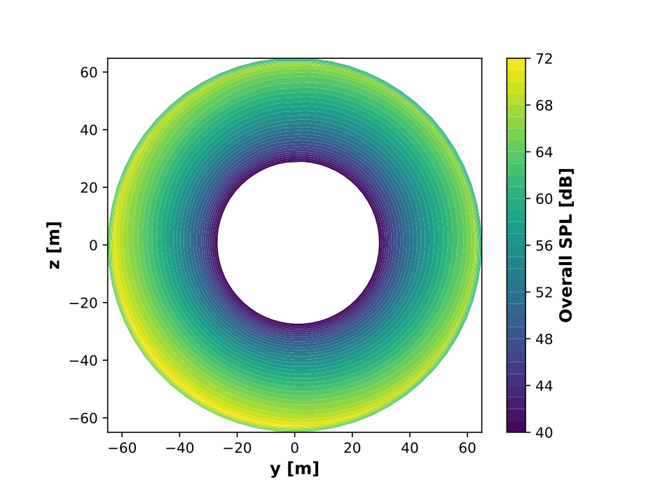
Fig. 4.24 Map of the overall SPL of the rotor of the reference wind turbine from Simplified Guidati and BPM TBL-TE noise models. The observer is located 175 meters downwind at a height of 2 meters.

2

https://github.com/NREL/ROSCO

3

https://github.com/OpenFAST/python-toolbox