4.12.1. Input Files
The user configures the sea state model parameters via a primary SeaState input file. When used in standalone mode, an additional driver input file is required. This driver file specifies initialization inputs normally provided to SeaState by OpenFAST.
No lines should be added or removed from the input files, except in tables where the number of rows is specified.
4.12.1.1. Units
SeaState uses the SI system (kg, m, s).
4.12.1.2. SeaState Driver Input File
The driver input file is only needed for the standalone version of SeaState and contains inputs normally generated by OpenFAST. It is necessary to control the sea state conditions for uncoupled models. An example SeaState driver input file is given in Appendix B.
Set the Echo flag in this file to TRUE if you wish to have
SeaStateDriver echo the contents of the driver input file (useful
for debugging errors in the driver file). The echo file has the naming
convention of OutRootName.dvr.ech. OutRootName is specified
in the SEASTATE section of the driver input file. Set the gravity
constant using the Gravity parameter. SeaState expects a magnitude,
so in SI units this would be set to 9.80665 \(\frac{m}{s^{2}}\).
WtrDens specifies the water density and must be a value greater than
or equal to zero; a typical value for seawater is around 1025
kg/m3. WtrDpth specifies the water depth (depth of the flat
seabed) relative to the MSL and must be a value greater than
zero. MSL2SWL is the offset between the MSL and SWL, positive if SWL
is above MSL. SeaStateInputFile is the filename of the primary SeaState
input file. This name should be in quotations and can contain an absolute
path or a relative path.
WrWvKinMod controls the wave kinematics output from the SeaState driver. Setting it to 0 suppresses driver output of wave kinematics. The driver will output the wave-elevation time series at the global origin (0,0) in a separate .Elev file if WrWvKinMod = 1. This file also serves as a valid WvKinFile for WaveMod = 5 (externally generated wave-elevation time series) in the primary SeaState input file. If WrWvKinMod = 2, SeaState will output the full wave kinematics (velocity, acceleration, dynamic pressure, and wave elevation) at all wave grid points in eight output files with the extensions .Vxi, .Vyi, .Vzi, .Axi, .Ayi, .Azi, .DynP, and .Elev. The velocity and acceleration outputs are all in the global earth-fixed coordinate system. These files are also valid as WvKinFile for WaveMod = 6 (externally generated full wave-kinematics time series) and can be used as templates if the users would like to build their own input files for WaveMod = 6. NSteps specifies the number of simulation time steps, and TimeInterval specifies the time between steps. WaveElevSeriesFlag can be set to TRUE to output a file with the extension .WaveElev.out, which contains the wave-elevation field at each time step for visualization purposes. Setting it to FALSE suppresses this output. Note that the grid points for WrWvKinMod = 2 and WaveElevSeriesFlag = TRUE are both controlled by the SPATIAL DISCRETIZATION section of the primary SeaState input file explained below.
4.12.1.3. SeaState Primary Input File
An example SeaState primary input file is given in Appendix A.
4.12.1.3.1. Environmental Conditions
Environmental conditions are now specified in the driver input file but are left in the primary input file for legacy compatibility. Use the keyword DEFAULT to pass in values specified by the driver input file. Otherwise, values given in the primary input file will overwrite those given in the driver input file. WtrDens specifies the water density and must be a value greater than or equal to zero; a typical value of seawater is around 1025 kg/m3. WtrDpth specifies the water depth (depth of the flat seabed), based on the reference MSL, and must be a value greater than zero. MSL2SWL is the offset between the MSL and SWL, positive when SWL is above MSL. This parameter is useful when simulating the effect of tides or storm-surge sea-level variations without having to alter the substructure geometry information. This parameter is unused with WaveMod = 6 and must be set to zero if you are using a potential-flow model (PotMod = 1 or 2) in HydroDyn.
4.12.1.3.2. Spatial discretization
The SPATIAL DISCRETIZATION section controls the generation of a wave grid. This wave grid is used primarily by HydroDyn but also by other modules of OpenFAST to compute the hydrodynamic and hydrostatic loads on structures in water. The wave grid is added to allow strip-theory members in HydroDyn to use the wave kinematics and dynamic pressure at the instantaneous displaced position of the structure when evaluating the loads. It also allows the potential-flow wave excitation in HydroDyn to be corrected based on any large drift motion in the horizontal plane, such as that due to high wind thrust.
Note that in previous versions of OpenFAST, the potential-flow wave excitation and wave field for strip-theory members were precomputed with the structure at the undisplaced position. This mode of operation is no longer present in OpenFAST, and a wave grid must always be defined even if the user chooses not to account for structure displacement when evaluating the strip-theory and/or potential-flow hydrodynamic loads in HydroDyn.
Currently, the SeaState wave grid is always centered at the global origin and symmetric about the XZ-plane and YZ-plane.
X_HalfWidth sets (in m) the half width of the wave grid in the global X-direction, such that the wave grid covers the region of −X_HalfWidth ≤ X ≤ +X_HalfWidth. X_HalfWidth must be greater than zero.
Y_HalfWidth sets (in m) the half width of the wave grid in the global Y-direction, such that the wave grid covers the region of −Y_HalfWidth ≤ Y ≤ +Y_HalfWidth. Y_HalfWidth must be greater than zero.
Z_Depth sets the depth (in m) of the wave grid, such that the wave grid covers the region of (MSL2SWL − Z_Depth) ≤ Z ≤ MSL2SWL. Z_Depth must be greater than zero and less than or equal to MSL2SWL + WtrDpth. Setting Z_Depth to DEFAULT will automatically set its value to MSL2SWL + WtrDpth.
NX sets the number of uniformly distributed grid points in the X-direction over half of the domain, including a point at the origin. Therefore, the total number of grid points in the X-direction is equal to 2NX−1. NX must be greater than or equal to 2.
NY sets the number of uniformly distributed grid points in the Y-direction over half of the domain, including a point at the origin. Therefore, the total number of grid points in the Y-direction is equal to 2NY−1. NY must be greater than or equal to 2.
NZ sets the number of grid points in the vertical Z-direction from Z = (MSL2SWL − Z_Depth) to Z = MSL2SWL. The distribution of grid points in the Z-direction is not uniform. It instead follows a cosine distribution: Z[n] = Z_Depth(cos(n·dθ)–1), where n = 0,1,…,NZ-1 and dθ = π/(2(NZ-1)). This distribution places more grid points near the free surface. NZ must be greater than or equal to 2.
When setting up the wave grid, it is necessary to make sure the wave grid is large enough in all three directions, so that no part of the structure defined in HydroDyn moves out of the wave grid during the simulation. At the same time, the grid should also be fine enough to resolve the shortest wave of interest.
OpenFAST precomputes and saves the wave-field velocity, acceleration, dynamic pressure, and wave elevation at the start of the simulation. Generating and maintaining the wave grid can be memory intensive for long simulations. Users should set the wave grid to be no larger or finer than necessary to reduce memory use. Reducing WaveTMax or increasing WaveDT (see WAVES section below) also reduces memory use. For long crested waves (no directional spreading) aligned with the X-direction (or Y-direction), NY (or NX) can be reduced to the minimum allowed value of 2 to save memory.
4.12.1.3.3. Waves
The WAVES section of the input file controls the internal generation of first-order waves or the use of externally generated waves, used by both strip-theory and potential-flow modeling in HydroDyn. The wave spectrum settings in this section only pertain to the first-order wave frequency components. When second-order terms are optionally enabled—see the 2nd-Order Waves and 2nd-Order Floating Platform Forces sections below—the second-order terms are calculated using the first-order wave-component amplitudes and extra energy is added to the wave spectrum (at the difference and sum frequencies).
WaveMod specifies the incident wave kinematics model. The options are:
0: none = still water
1: regular (periodic) waves
1P#: regular (periodic) waves with user-specified phase, for example 1P20.0 for regular waves with a 20˚ phase (without P#, the phase will be random, based on WaveSeed); 0˚ phase represents a cosine function, starting at the peak and decreasing in time
2: Irregular (stochastic) waves based on the JONSWAP or Pierson-Moskowitz frequency spectrum
3: Irregular (stochastic) waves based on a white-noise frequency spectrum
4: Irregular (stochastic) waves based on a user-defined frequency spectrum from routine UserWaveSpctrm(); need to recompile the SeaState standalone program or OpenFAST.
5: Externally generated wave-elevation time series
6: Externally generated full wave-kinematics time series
7: User-defined wave frequency components
Option 4 requires that the UserWaveSpctrm() subroutine of the Waves.f90 source file be implemented by the user, and will require recompiling either the standalone SeaState program or OpenFAST. Option 5 allows the use of externally generated wave-elevation time series, from which the hydrodynamic loads in the potential-flow solution or the wave kinematics used in the strip-theory solution are derived internally. Option 6 allows the use of full externally generated wave kinematics for use with the strip-theory solution (but not the potential-flow solution). Option 7 allows the user to specify wave frequency components (amplitude/wave height, phase, and heading). With options 5, 6, and 7, the externally generated wave data is provided through input files, all of which have the root name given by the WvKinFile parameter below.
WaveStMod sets the wave-stretching formulation, which allows strip- theory hydrodynamic and hydrostatic loads (with wave-slope contribution) to be evaluated up to the instantaneous incident-wave free surface in HydroDyn. Currently, three different wave-stretching formulations are implemented: vertical stretching (option 1), extrapolation stretching (option 2), and Wheeler stretching (option 3). Using any of the three wave-stretching models will also result in HydroDyn computing the nonlinear hydrostatic load on strip-theory members up to the instantaneous free surface, including any contribution from non-zero wave slope. Setting WaveStMod to 0 disables wave stretching, and the strip-theory hydrodynamic and hydrostatic loads will always be evaluated up to the SWL. Extrapolation stretching (WaveStMod = 2) is not supported when WaveMod = 6 (externally generated full wave-kinematics time series).
WvCrntMod controls the modeling of combined wave and current conditions. It can be set to 0, 1, or 2 with the following effects.
WvCrntMod value |
Effects |
|---|---|
0 |
Simple superposition where the current velocity and acceleration are added to those of the waves. Current has no direct impact on the waves. This option reproduces the behavior of previous versions of OpenFAST. |
1 |
Include Doppler effect on the waves by solving the wave dispersion relation corrected for current. The input wave spectrum/time series are assumed to be those directly measured in a region with the current and are not modified by SeaState. Wavelengths are corrected for Doppler effect. |
2 |
Full interaction between waves and current with both Doppler effect and wave amplitude/spectrum scaling for wave-current interactions. The input wave spectrum/time series are assumed to be those measured in a region without current and rescaled based on the current velocity/direction. |
Setting WvCrntMod to 1 and 2 imposes additional restrictions on the allowed waves and current.
WvCrntMod value |
Restrictions |
|---|---|
0 |
No additional restrictions |
1 |
First-order long-crested waves without directional spreading |
2 |
First-order long-crested waves without directional spreading; colinear (aligned or opposing) waves and current only; the amplitude/spectrum scaling implemented assumes deep-water conditions, although this is not checked. |
Strictly speaking, options 1 and 2 of WvCrntMod are only valid for a uniform current; however, sheared current is allowed, and it is up to the user to ensure that the current profile near the surface down to a depth relevant to the waves is reasonably uniform. SeaState simply takes the current velocity at the still water level when computing the effects of the current on the waves. The improved wave-current modeling can be used with either SeaState current or dynamic current from InflowWind when simulating marine hydrokinetic turbines. For the latter, wave-current interaction is based on the time-averaged current velocity at the still water level. For applicable WindType in InflowWind, users should ensure that the flow-field grid from InflowWind reaches the still water level. WvCrntMod has no effect when WaveMod = 0 or 6, or when there is no current from either SeaState (CurrMod = 0) or InflowWind if simulating marine hydrokinetic turbines.
WaveTMax sets the length of the incident wave kinematics time series, but it also determines the frequency step used in the inverse FFT, from which the internal wave time series are derived (Δω = 2π/WaveTMax). When WaveMod = 7 (user-defined wave frequency components), all frequency components specified by the user must be integer multiples of Δω with the lowest allowed frequency being equal to Δω. If WaveTMax is less than the total simulation time, SeaState implements repeating wave kinematics that have a period of WaveTMax; WaveTMax must not be less than the total simulation time when WaveMod = 5. WaveDT determines the time step for the wave kinematics time series, but it also determines the maximum frequency in the inverse FFT (ωmax = π/WaveDT). When WaveMod = 7, WaveDT is not used, and the appropriate time step is determined internally based on the user-defined frequency components. When modeling irregular sea states, we recommend that WaveTMax be set to at least 1 hour (3600 s) and that WaveDT be a value in the range between 0.1 and 1.0 s to ensure sufficient resolution of the wave spectrum and wave kinematics. When SeaState is coupled to OpenFAST, WaveDT may be specified arbitrarily independently from the glue code time step of OpenFAST (wave kinematics will be interpolated in time as necessary); WaveDT must equal the glue code time step of OpenFAST when WaveMod = 6. WaveTMax and WaveDT also affect the amount of memory used by the SeaState wave grid; a shorter WaveTMax and a longer WaveDT reduce memory use.
For internally generated waves, the wave height (crest-to-trough, twice the amplitude) for regular waves and the significant wave height for irregular waves are set using WaveHs (only used when WaveMod = 1, 2, or 3). The wave period for regular waves and the peak-spectral wave period for irregular waves is controlled with the WaveTp parameter (only used when WaveMod = 1 or 2). WavePkShp is the peak-shape parameter of JONSWAP irregular wave spectrum (only used when WaveMod = 2). Set WavePkShp to DEFAULT to obtain the value recommended in the IEC 61400-3 Annex B, derived based on the peak-spectral period and significant wave height [IEC, 2009]. Set WavePkShp to 1.0 for the Pierson-Moskowitz spectrum.
WvLowCOff and WvHiCOff control the lower and upper cut-off frequencies (in rad/s) of the first-order wave spectrum; the first-order wave-component amplitudes are zeroed below and above these cut-off frequencies, respectively. WvLowCOff may be set lower than the low-energy limit of the first-order wave spectrum to minimize computational expense. Setting a proper upper cut-off frequency (WvHiCOff) also minimizes computational expense and is important to prevent nonphysical effects when approaching of the breaking-wave limit and to avoid nonphysical wave forces at high frequencies (i.e., at short wavelengths) when using a strip-theory solution. WvLowCOff and WvHiCOff are unused when WaveMod = 0, 1, or 6.
WaveDir (unused when WaveMod = 0 or 6) is the mean wave propagation heading direction (in degrees), and must be in the range (-180,180]. A heading of 0 corresponds to wave propagation in the positive X-axis direction. And a heading of 90 corresponds to wave propagation in the positive Y-axis direction. WaveDirMod specifies the wave directional spreading model (only used when WaveMod = 2, 3, or 4). Setting WaveDirMod to 0 disables directional spreading, resulting in long-crested (plane-progressive) sea states propagating in the WaveDir direction. Setting WaveDirMod to 1 enables the modeling of short-crested sea states, with a mean propagation direction of WaveDir, through the commonly used cosine spreading function (COS:sup:2S) to define the directional spreading spectrum, based on the spreading coefficient (S) defined via WaveDirSpread. The wave directional spreading spectrum is discretized with an equal-energy method using WaveNDir number of equal-energy bins. WaveNDir is an odd-valued integer greater than or equal to 1 (1 or 3 or 5…), but SeaState may slightly increase the specified value of WaveNDir to ensure that there is the same number of wave components within each direction bin; setting WaveNDir = 1 is equivalent to setting WaveDirMod = 0. The range of the directional spread (in degrees) is defined via WaveDirSpread. The equal-energy method assumes that the directional spreading spectrum is the product of a frequency spectrum and a spreading function i.e. S(ω,β) = S(ω)D(β). Directional spreading is not permitted when using Newman’s approximation of the second-order difference-frequency potential-flow loads.
WaveSeed(1) and WavedSeed(2) (unused when WaveMod = 0, 5, or 1) combined determine the initial seed (starting point) for the internal pseudorandom number generator (pRNG) needed to derive the internal wave kinematics from the wave frequency and direction spectra. If both are numeric values, the Fortran intrinsic pRNG is used. If WaveSeed(2) is the string “RANLUX”, an alternative pRNG included with the NWTC Library is used and the value of WaveSeed(1) is the seed. If you want to run different time-domain realizations for given boundary conditions (of significant wave height, and peak-spectral period, etc.), you should change one or both seeds between simulations. While the phase of each wave frequency and direction component of the wave spectrum is always based on a uniform distribution (except when using the 1P# WaveMod option), the amplitude of the wave frequency spectrum can also be randomized (following a normal distribution) by setting WaveNDAmp to TRUE. Setting WaveNDAmp to FALSE means that the amplitude of the wave frequency spectrum always matches the target spectrum. WaveNDAmp is only used with WaveMod = 2, 3, or 4.
When using externally generated wave data (WaveMod = 5, 6, or 7), input parameter WvKinFile should be set to the root name of the input file(s) without extension when WaveMod = 5 or 6 or the full file name with extension when WaveMod = 7.
Using externally generated wave-elevation time series (WaveMod = 5) requires a text-formatted input data file with the extension .Elev containing two columns of data—the first is time (starting at zero) (in s) and the second is the wave elevation at (0,0) (in m), separated by whitespace. Header lines (identified as those not beginning with a number) are ignored. The time series must be at least WaveTMax in length and not less than the total simulation time, and the time step must match WaveDT. The wave-elevation time series specified is assumed to be of first order and long-crested, but is not checked for physical correctness. When second-order terms are optionally enabled—see the 2ND-ORDER WAVES section below—the second-order terms are calculated using the wave-component amplitudes derived from the provided wave-elevation time series and extra energy is added to the wave spectrum (at the difference and sum frequencies).
Using full externally generated wave kinematics (WaveMod = 6) requires eight text-formatted input data files, all without headers. Seven files with extensions .Vxi, .Vyi, .Vzi, .Axi, .Ayi, .Azi, and .DynP correspond to the X, Y, and Z velocities (in m/s) and accelerations (in m/s2) in the global inertial-frame coordinate system and the dynamic pressure (in Pa) time series. Each of these files must have 13 headerlines, which will be skipped by SeaState, followed by exactly WaveTMax/WaveDT rows and N whitepace-separated columns, where N is the total number of SeaState wave grid points (corresponding exactly to those written to the SeaState summary file). The nodes are ordered by incrementing the X-position first, followed by incrementing the Y-position, and finally incrementing the Z-position, as they appear in the SeaState summary file. The first node is located at (-X_HalfWidth,-Y_HalfWidth,MSL2SWL-Z_Dpth). Time is absent from the files but is assumed to go from zero to WaveTMax in steps of WaveDT. The eighth file, with extension .Elev, contains the wave-elevation time series (in m). This file must have exactly WaveTMax/WaveDT rows and as many whitepace-separated columns as there are grid nodes in a horizontal plane. The nodes are ordered by incrementing the X-position first followed by incrementing the Y-position. The first node is located at (-X_HalfWidth,-Y_HalfWidth). To use this feature, it is the burden of the user to generate wave kinematics data at each of SeaState’s time steps and grid points. SeaState will not interpolate the data when populating the wave grid. In these input files, a numeric value (including 0) in a file is assumed to be valid data (with 0 corresponding to 0 m, 0 m/s, 0 m/s2, or 0 Pa); a nonnumeric string will be converted to a zero. The data in these files is not processed (filtered, etc.) or checked for physical correctness. Full externally generated wave kinematics (WaveMod = 6) cannot be used in conjunction with the potential-flow solution, and only vertical and Wheeler wave stretching are allowed, not extrapolation stretching. Users can run the SeaState standalone driver program with any of the internal wave-generation models, e.g., WaveMod = 2, with WrWvKinMod = 2 in the driver input to generate a set of valid input files for WaveMod = 6 as templates.
Using user-defined wave frequency components (WaveMod = 7) requires a text-formatted input data file with the extension .Comp containing four columns of data. The first column contains the angular frequency (in rad/s) of the wave component, the second is the peak-to-trough wave height (in m) of the component, the third is the wave heading of the component following the convention of WaveDir above (in deg), and the last column is the wave phase of the frequency component (in deg). A phase of zero corresponds to a wave crest at the global origin at t = 0. The four columns are separated by whitespaces. Header lines (identified as those not beginning with a number) are ignored. A valid input file must meet the following requirements:
All frequency entries must be integer multiples of the frequency step, Δω = 2π/WaveTMax. A relative tolerance of 10-3 is enforced to allow for some truncation errors in the input frequencies. Users should make sure the input frequencies and WaveTMax contain enough significant digits to meet this requirement. The lowest allowed wave angular frequency is Δω.
If a frequency component has zero wave height, it can be omitted from the input file.
The frequency components listed in the input file need not be in any particular order.
For each frequency, there can only be one entry. It is not allowed, for example, to have two wave components with different headings but the same frequency.
The wave components specified are assumed to be of first order and long-crested, but are not checked for physical correctness. When second-order terms are optionally enabled—see the 2ND-ORDER WAVES section below—the second-order terms are calculated using the wave components specified and extra energy is added to the wave spectrum (at the difference and sum frequencies).
4.12.1.3.4. 2nd-Order Waves
The 2ND-ORDER WAVES section (unused when WaveMod = 0 or 6) of the input file allows the option of adding second-order contributions to the wave kinematics used by the strip-theory solution. When second-order terms are optionally enabled, the second-order terms are calculated using the first-order wave-component amplitudes and extra energy is added to the wave spectrum (at the difference and sum frequencies). The second-order terms cannot be computed without also including the first-order terms from the WAVES section above. Enabling the second-order terms allows one to capture some of the nonlinearities of real surface waves, permitting more accurate modeling of sea states and the associated wave loads at the expense of greater computational effort (mostly at SeaState initialization).
While the cut-off frequencies in this section apply to both the second-order wave kinematics from SeaState (used for strip-theory loads in HydroDyn) and the second-order potential-flow loads in HydroDyn, the second-order terms themselves are enabled separately. The second-order wave kinematics used by strip theory are enabled in this section, while the second-order diffraction loads from potential-flow theory are enabled in the 2nd-Order Floating Platform Forces section of the primary HydroDyn input file. The wave elevation outputs from SeaState will only include the second-order contributions when the second-order wave kinematics are enabled in this section.
To use second-order wave kinematics in the strip-theory solution, set WvDiffQTF and/or WvSumQTF to TRUE. When WvDiffQTF is set to TRUE, second-order difference-frequency terms, calculated using the full difference-frequency QTF, are incorporated in the wave kinematics. When WvSumQTF is set to TRUE, second-order sum-frequency terms, calculated using the full sum-frequency QTF, are incorporated in the wave kinematics. The full difference- and sum-frequency wave kinematics QTFs are implemented analytically following [Sharma and Dean, 1981], which extends Stokes second-order theory to irregular multidirectional waves. A setting of FALSE disregards the second-order contributions to the wave kinematics in the strip-theory solution.
WvLowCOffD and WvHiCOffD control the lower and upper cut-off frequencies (in rad/s) of the second-order difference-frequency terms; the second-order difference-frequency terms are zeroed below and above these cut-off frequencies, respectively. The cut-offs apply directly to the physical difference frequencies, not the two individual first-order frequency components leading to the difference frequencies. When enabling second-order potential-flow loads in HydroDyn, a setting of WvLowCOffD = 0 is advised to avoid eliminating the mean-drift term (second-order wave kinematics do not have a nonzero mean). WvHiCOffD need not be set higher than the peak-spectral frequency of the first-order wave spectrum (ωp = 2π/WaveTp) to minimize computational expense.
Likewise, WvLowCOffS and WvHiCOffS control the lower and upper cut-off frequencies (in rad/s) of the second-order sum-frequency terms; the second-order sum-frequency terms are zeroed below and above these cut-off frequencies, respectively. The cut-offs apply directly to the physical sum frequencies, not the two individual first-order frequency components leading to the sum frequencies. WvLowCOffS need not be set lower than the peak-spectral frequency of the first-order wave spectrum (ωp = 2π/WaveTp) to minimize computational expense. Setting a proper upper cut-off frequency (WvHiCOffS) also minimizes computational expense and is important to (1) ensure convergence of the second-order summations, (2) avoid unphysical “bumps” in the wave troughs, (3) prevent nonphysical effects when approaching of the breaking-wave limit, and (4) avoid nonphysical wave forces at high frequencies (i.e., at short wavelengths) when using a strip-theory solution.
Because the second-order terms are calculated using the first-order wave-component amplitudes, the second-order cut-off frequencies (WvLowCOffD, WvHiCOffD, WvLowCOffS, and WvHiCOffS) are used in conjunction with the first-order cut-off frequencies (WvLowCOff and WvHiCOff) from the WAVES section. However, the second-order cut-off frequencies are not used by Newman’s approximation of the second-order difference-frequency potential-flow loads, which are derived solely from first-order effects.
4.12.1.3.5. Constrained wave
The CONSTRAINED WAVE section allows the user to prescribe and embed a large wave crest in JONSWAP stochastic waves (WaveMod = 2), following the constrained NewWave method of Taylor, Jonathan, and Harland (1997).
ConstWaveMod can be set to 0 for no embedded wave, 1 for embedded wave with prescribed crest elevation from SWL, or 2 for embedded wave with prescribed crest-to-trough wave height.
CrestHmax (in m) is twice the crest elevation from SWL if ConstWaveMod = 1 or the crest-to-trough wave height if ConstWaveMod = 2. CrestHmax must be greater than WaveHs.
CrestTime is the time (in s) from the start of the simulation at which the user-prescribed wave crest is to occur.
CrestXi is the X-position (in m) of the embedded wave crest in the global frame of reference.
CrestYi is the Y-position (in m) of the embedded wave crest in the global frame of reference.
Constrained wave is only compatible with WaveMod = 2 (JONSWAP wave spectrum). If WaveMod is set to other values, this section of the input file will be ignored.
In the absence of second-order wave components, the crest elevation or crest height will match the user input CrestHmax exactly. If second-order wave components are included by setting either WvDiffQTF or WvSumQTF to TRUE, the resulting crest elevation or crest height can deviate from CrestHmax.
4.12.1.3.6. Current
You can include water velocity due to a current model by setting CurrMod = 1. If CurrMod is set to zero, then the simulation will not include current. CurrMod = 2 requires that the UserCurrent() subroutine of the Current.f90 source file be implemented by the user, and will require recompiling either the standalone SeaState program or OpenFAST. Current induces steady hydrodynamic loads through the viscous-drag terms (both distributed and lumped) of strip-theory members in HydroDyn. Current is not used in the potential-flow solution or when WaveMod = 6.
SeaState’s standard current model includes three sub-models: near-surface, sub-surface, and depth-independent, as illustrated in Fig. 4.50. All three currents are vector summed, along with the wave particle kinematics velocity.
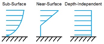
Fig. 4.50 Standard Current Sub-Models
The sub-surface current model follows a power law,
where \(Z\) is the local depth below the SWL (negative downward), \(d\) is the water depth (equal to WtrDpth + MSL2SWL), and \(U_{0_{SS}}\) is the current velocity at SWL, corresponding to CurrSSV0. The heading of the sub-surface current is defined using CurrSSDir following the same convention as WaveDir.
The near-surface current model follows a linear relationship down to a reference depth such that,
otherwise,
where \(h_{ref}\) is the reference depth corresponding to CurrNSRef and must be positive valued. \(U_{0_{NS}}\) is the current velocity at SWL, corresponding to CurrNSV0. The heading of the near-surface current is defined using CurrNSDir, following the same convention as WaveDir.
The depth-independent current velocity everywhere equals CurrDIV. This current has a heading direction CurrDIDir, following the same convention as WaveDir.
4.12.1.3.7. MacCamy-Fuchs diffraction model
HydroDyn now supports the MacCamy-Fuchs wave-diffraction solution for strip-theory members. This option attenuates the strip-theory wave excitation when the wavelength is comparable to or smaller than the member diameter, thus providing more realistic loads at higher frequencies. To limit memory use, the current OpenFAST implementation requires all strip-theory members in HydroDyn that uses the MacCamy-Fuchs diffraction solution to have diameters within +/-10% of a reference diameter given by MCFD here. If MacCamy-Fuchs diffraction solution is not used in HydroDyn, set MCFD to a number less than or equal to zero to reduce memory use and SeaState initialization time.
4.12.1.3.8. Output Channels
This section controls output quantities generated by SeaState. Enter one or more lines containing quoted strings that in turn contain one or more output parameter names. Separate output parameter names by any combination of commas, semicolons, spaces, and/or tabs. If you prefix a parameter name with a minus sign, “-“, underscore, “_”, or the characters “m” or “M”, SeaState will multiply the value for that channel by –1 before writing the data. The parameters are not necessarily written in the order they are listed in the input file. SeaState allows you to use multiple lines so that you can break your list into meaningful groups and so the lines can be shorter. You may enter comments after the closing quote on any of the lines. Entering a line with the string “END” at the beginning of the line or at the beginning of a quoted string found at the beginning of the line will cause SeaState to quit scanning for more lines of channel names. If SeaState encounters an unknown/invalid channel name, it warns the users but will remove the suspect channel from the output file. Please refer to Appendix C for a complete list of possible output parameters.
You can generate up to 9 wave elevation outputs. NWaveElev determines the number (between 0 and 9), and the whitespace-separated lists of WaveElevxi and WaveElevyi determine the locations of these NWaveElev number of points in the global inertial-frame coordinate system.
You can also specify up to 9 locations in space to output wave kinematics (fluid velocity and acceleration) and dynamic pressure. NWaveKin determines the number (between 0 and 9), and the whitespace-separated lists of WaveKinxi, WaveKinyi, and WaveKinzi determine the locations of these NWaveKin number of points in the global inertial-frame coordinate system. If one of the wave-stretching model is selected, its effect will be reflected in the wave kinematics and dynamic pressure outputs. For example, a point below SWL will report all zeros if it is momentarily out of water due to a wave trough. Similarly, a point above SWL will report wave kinematics and dynamic pressure according to the wave-stretching model selected if it is momentarily in water due to a wave crest. Any point out of water will report zeros in all wave-kinematics and dynamic-pressure outputs until it reenters water.