4.19.7. FAST.Farm Theory
FAST.Farm is a multiphysics engineering tool for predicting the performance and loads of wind turbines within a wind farm. FAST.Farm uses OpenFAST to solve the aero-hydro-servo-elastic dynamics of each individual turbine, but considers additional physics for wind-farm-wide ambient wind in the atmospheric boundary layer; and wake deficits, advection, deflection, meandering, and merging. FAST.Farm is based on the principles of the DWM model – including passive tracer modeling of wake meandering – but addresses many of the limitations of previous DWM implementations.
4.19.7.1. Dynamic Wake Meandering Principles and Limitations Addressed
The main idea behind the DWM model is to capture key wake features pertinent to accurate prediction of wind farm power performance and wind turbine loads, including the wake-deficit evolution (important for performance) and the wake meandering and wake-added turbulence (important for loads, see Section 4.19.7.2.3.4). Although fundamental laws of physics are applied, appropriate simplifications have been made to minimize the computational expense, and HFM solutions are used to inform and calibrate the submodels. In the DWM model, the wake-flow processes are treated via the “splitting of scales,” in which small turbulent eddies (less than two diameters) affect wake-deficit evolution and large turbulent eddies (greater than two diameters) affect wake meandering.
The presence of thrust from the wind turbine rotor causes the wind speed to decrease and the pressure to increase just upwind of the rotor. In the near-wake region just downwind of the rotor – illustrated in Fig. 4.66 – coherent vortices break down, the pressure recovers to free stream, the wind speed decreases further, and the wake expands radially. In the far-wake region further downwind, the wake deficit is approximately Gaussian and recovers to free stream due to the turbulent transfer of momentum into the wake from the ambient wind across the wake shear layer. This flow-speed reduction and gradual recovery to free stream is known as the wake-deficit evolution. In most DWM implementations, the wake-deficit evolution is modeled via the thin shear-layer approximation of the Reynolds-averaged Navier-Stokes equations under quasi-steady-state conditions in axisymmetric coordinates – illustrated in Fig. 4.58. The turbulence closure is captured by using an eddy-viscosity formulation, dependent on small turbulent eddies. This wake-deficit evolution solution is only valid in the far wake. This far wake is most important for wind farm analysis because wind turbines are not typically spaced closely. However, because the wake-deficit evolution solution begins at the rotor, a near-wake correction is applied at the inlet boundary condition to improve the accuracy of the far-wake solution.
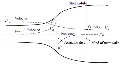
Fig. 4.66 Near-wake region.
Wake meandering is the large-scale movement of the wake deficit transported by large turbulent eddies. This wake-meandering process is treated pragmatically in DWM ([ff-Leal08]) by modeling the meandering as a passive tracer, which transfers the wake deficit transversely (horizontally and vertically) to a moving frame of reference (MFoR) – as illustrated in Fig. 4.55 – based on the ambient wind (including large turbulent eddies) spatially averaged across planes of the wake.
Wake-added turbulence is the additional small-scale turbulence generated from the turbulent mixing in the wake. It is often modeled in DWM by scaling up the background (undisturbed) turbulence (see Section 4.19.7.2.3.4).
Several variations of DWM have been implemented, e.g., by the Technical University of Denmark ([ff-Meal10, ff-Meal16]) and the University of Massachusetts ([ff-Ceal15, ff-Hao16, ff-Heal14]). Although the exact limitations of existing DWM implementations depend on the implementation, specific limitations that are addressed in developing FAST.Farm are summarized in Table 4.15 and are discussed where appropriate in the next section.
Limitation |
Solution/Innovation |
|---|---|
|
|
|
|
|
|
|
|
|
|
|
|
4.19.7.2. FAST.Farm Theory Basis
FAST.Farm is a nonlinear time-domain multiphysics engineering tool composed of multiple submodels, each representing different physics domains of the wind farm. FAST.Farm is implemented as open-source software that follows the programming requirements of the FAST modularization framework ([ff-Jon13]), whereby the submodels are implemented as modules interconnected through a driver code. The submodel hierarchy of FAST.Farm is illustrated in Fig. 4.56. Wake advection, deflection, and meandering; near-wake correction; and wake-deficit increment are submodels of the wake-dynamics (WD) model, implemented in a single module. Ambient wind and wake merging are submodels of the ambient wind and array effects (AWAE) model, implemented in a single module. Combined with the OpenFAST (OF) modules, FAST.Farm has three modules and one driver. There are multiple instances of the OF and WD modules – one instance for each wind turbine/rotor. Each submodel/module is described in the subsections below.
FAST.Farm can be compiled and run in serial or parallel mode. Parallelization has been implemented in FAST.Farm through OpenMP, which allows FAST.Farm to take advantage of multicore computers by dividing computational tasks among the cores/threads within a node (but not between nodes) to speed up a single simulation. This process is illustrated in Fig. 4.67 for a node where the number of threads (\(N_{Th}\)) is greater than the number of wind turbines (\(N_t\)). There is one instance of the AWAE modules and \(N_t\) instances of the OF and WD modules. The initialization, update states, calculate output, and end calls to each module are shown. The output calculation of AWAE is parallelized across all threads. During time marching, each instance of OF is solved in parallel while the ambient wind data are read by AWAE.
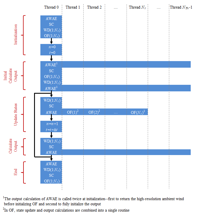
Fig. 4.67 FAST.Farm parallelization process.
The size of the wind farm and number of wind turbines is limited only by the available RAM. In parallel mode, each instance of the OpenFAST submodel can be run in parallel on separate threads. At the same time, the ambient wind within the AWAE module is being read into memory on another thread. Thus, the fastest simulations require at least one more core than the number of wind turbines in the wind farm. Furthermore, the output calculations within the AWAE module are parallelized into separate threads. To support the modeling of large wind farms, single simulations involving memory parallelization and parallelization between nodes of a multinode HPC through MPI is likely required. MPI has not yet been implemented within FAST.Farm. However, a multinode HPC can be used to run multiple serial or parallelized simulations in parallel (in batch mode) on separate nodes. In serial mode, multiple serial simulations can be run in parallel (in batch mode) on separate cores and/or nodes.
4.19.7.2.1. FAST.Farm Driver
The FAST.Farm driver, also known as the “glue code,” is the code that couples individual modules together and drives the overall time-domain solution forward. Additionally, the FAST.Farm driver reads an input file of simulation parameters, checks the validity of these parameters, initializes the modules, writes results to a file, and releases memory at the end of the simulation.
To simplify the coupling algorithm in the FAST.Farm driver and ensure computational efficiency, all module states (\(x^d\)), inputs (\(u^d\)), outputs (\(y^d\)), and functions (\(X^d\) for state updates and \(Y^d\) for outputs) in FAST.Farm are expressed in discrete time, \(t=n\Delta t\), where \(t\) is time, \(n\) is the discrete-time-step counter, and \(\Delta t\) is the user-specified discrete time step (increment). Thus, the most general form of a module in FAST.Farm is simpler than that permitted by the FAST modularization framework ([ff-Jon13]), represented mathematically as: 1
The OF, and WD modules do not have direct feedthrough of input to output, meaning that the corresponding output functions simplify to \(y^d\left[ n \right]=Y^d\left( x^d\left[ n \right],n \right)\). The ability of the OF module to be written in the above form is explained in Section 4.19.7.2.2. Additionally, the AWAE module does not have states, reducing the module to a feed-forward-only system and a module form that simplifies to \(y^d\left[ n \right]=Y^d\left( u^d\left[ n \right],n \right)\). For functions in this manual, square brackets \(\left[\quad\right]\) denote discrete functions and round parentheses \(\left(\quad\right)\) denote continuous functions; the brackets/parentheses are dropped when implied. The states, inputs, and outputs of each of the FAST.Farm modules (OF, WD, and AWAE) are listed in Table 4.16 and explained further in the sections below.
Module |
States (Discrete Time) |
Inputs |
Outputs |
|---|---|---|---|
OpenFAST (OF) |
|
|
|
Wake Dynamics (WD) |
For \(0 \le n_p \le N_p-1\):
|
|
For \(0 \le n_p \le N_p-1\):
|
Ambient Wind and Array Effects (AWAE) |
|
For each turbine and \(0 \le n_p \le N_p-1\):
|
For each turbine:
|
After initialization and within each time step, the states of each module (OF, and WD) are updated (from time \(t\) to time \(t+\Delta t\), or equivalently, \(n\) to \(n+1\)); time is incremented; and the module outputs are calculated and transferred as inputs to other modules. Because of the form simplifications, the state updates of each module can be solved in parallel; the output-to-input transfer does not require a large nonlinear solve; and overall correction steps of the solution are not needed. The lack of a correction step is a major simplification of the coupling algorithm used within OpenFAST ([ff-Seal14, ff-Seal15]). Furthermore, the output calculations of the OF, and WD modules can be parallelized, followed then by the output calculation of the AWAE module. 2 In parallel mode, parallelization has been implemented in FAST.Farm through OpenMP.
Because of the small timescales and sophisticated physics, the OpenFAST submodel is the computationally slowest of the FAST.Farm modules. Additionally, the output calculation of the AWAE module is the only major calculation that cannot be solved in parallel to OpenFAST. Because of this, the parallelized FAST.Farm solution at its fastest may execute only slightly more slowly than stand-alone OpenFAST simulations. This results in simulations that are computationally inexpensive enough to run the many simulations necessary for wind turbine/farm design and analysis.
4.19.7.2.2. OpenFAST (OF Module)
FAST.Farm makes use of OpenFAST to model the dynamics (loads and motions) of distinct turbines in the wind farm. OpenFAST captures the environmental excitations (wind inflow; for offshore systems, waves, current, and ice) and coupled system response of the full system (the rotor, drivetrain, nacelle, tower, controller; for offshore systems, the substructure and station-keeping system). OpenFAST itself is an interconnection of various modules, each corresponding to different physical domains of the coupled aero-hydro-servo-elastic solution. The details of the OpenFAST solution are outside the scope of this document, but can be found in the hyperlink above and associated references.
The OF module of FAST.Farm is a wrapper that enables the coupling of OpenFAST to FAST.Farm – similar to the OpenFAST wrapper available in SOWFA, but with different inputs and outputs (described below). This wrapper also controls subcycling of the OpenFAST state updates. The timescales solved within OpenFAST are much smaller than those within FAST.Farm. Therefore, for accuracy and numerical stability reasons, the OpenFAST time step is typically much smaller than that required of FAST.Farm, as depicted in Fig. 4.68.
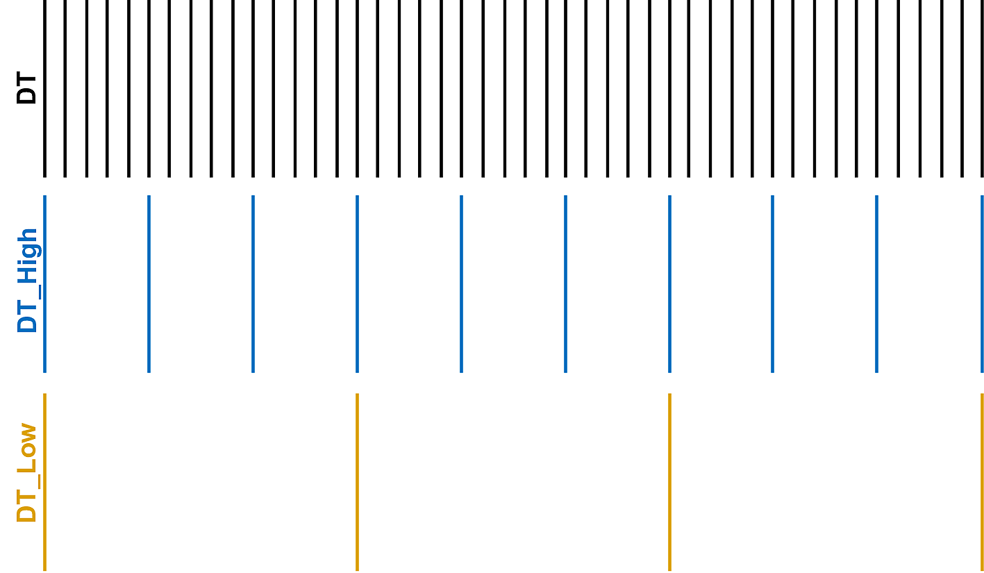
Fig. 4.68 Illustration of timescale ranges for OpenFAST (DT), the FAST.Farm high-resolution domain (DT_High), and the FAST.Farm low-resolution domain (DT_Low).
There is one instance of the OF module for each wind turbine. In parallel mode, these instances are parallelized through OpenMP. OpenFAST itself has various modules with different inputs, outputs, states, and parameters – including continuous-time, discrete-time, algebraic, and other (e.g., logical) states. However, for the purposes of coupling OpenFAST to FAST.Farm, the OF module functions in discrete time and without direct feedthrough of input to output. This is achieved by calling the OF module at the rate dictated by the FAST.Farm time step, \(\Delta t\), and by introducing a one-time-step (\(\Delta t\)) delay of the output relative to the input; this one-time-step delay is not expected to be problematic because of the slow timescales solved within FAST.Farm.
At initialization, the number of wind turbines (\(N_t\), with \(n_t\) the turbine counter such that \(1\le n_t\le N_t\)), the corresponding OpenFAST primary input files, and turbine origins in the global X-Y-Z inertial-frame coordinate system are specified by the user. Turbine origins are defined as the intersection of the undeflected tower centerline and the ground or, for offshore systems, mean sea level. The global inertial-frame coordinate system is defined with Z directed vertically upward (opposite gravity), X directed horizontally nominally downwind (along the zero-degree wind direction), and Y directed horizontally transversely.
The OF module also uses the disturbed wind (ambient plus wakes of neighboring turbines) across a high-resolution wind domain (in both time and space) around the turbine (output from the AWAE module – see Section 4.19.7.2.4 for more information), \(\vec{V}_\text{Dist}^\text{High}\), as input, to ensure that the individual turbine loads and response calculated by OpenFAST are accurately driven by flow through the wind farm, including wake and array effects. Spatially, the high-resolution wind domain must be large enough to encompass yawing of the rotor, blade deflection, and motion of the support structure (the latter is especially important for floating offshore wind turbines). OpenFAST uses a four-dimensional (three space dimensions plus one time dimension) interpolation to determine the wind local to its analysis nodes.
The OF module computes several outputs needed for calculating wake dynamics (inputs to the WD module). These include:
\(\hat{x}^\text{Disk}\) – the orientation of the rotor centerline
\(\vec{p}^\text{Hub}\) – the global position of the rotor center
\(D^\text{Rotor}\) – the rotor diameter
\(\gamma^\text{YawErr}\) – the nacelle-yaw error of the rotor
\(^\text{DiskAvg}V_x^\text{Rel}\) – the rotor-disk-averaged relative wind speed (ambient plus wakes of neighboring turbines plus turbine motion), normal to the disk
\(^\text{AzimAvg}C_t\left( r \right)\) – the azimuthally averaged thrust-force coefficient (normal to the rotor disk), distributed radially, where \(r\) is the radius.
In this manual, an over arrow (\(\vec{\quad}\)) denotes a three-component vector and a hat (\(\hat{\quad}\)) denotes a three-component unit vector. For clarity in this manual, \(\left( r \right)\) is used to denote radial dependence as a continuous function, even though the radial dependence is stored/computed on a discrete radial finite-difference grid within FAST.Farm. Except for \(\gamma^\text{YawErr}\) and \(^\text{AzimAvg}C_t\left( r \right)\), all of the listed variables were computed within OpenFAST before the development of FAST.Farm. \(\gamma^\text{YawErr}\) is defined as the angle about global Z from the rotor centerline to the rotor-disk-averaged relative wind velocity (ambient plus wakes of neighboring turbines plus turbine motion), both projected onto the horizontal global X-Y plane – see Fig. 4.57 for an illustration. \(^\text{AzimAvg}C_t\left( r \right)\) is computed by Equation (4.228)
where:
\(N_b\) – number of rotor blades, with \(n_b\) as the blade counter such that \(1\le n_b\le N_b\)
\(\left\{ \quad \right\}^T\) – vector transpose
\(\rho\) – air density
\(\vec{f}_{n_b}\left( r \right)\) – aerodynamic applied loads 3 distributed per unit length along a line extending radially outward in the plane of the rotor disk for blade \(n_b\).
The numerator of Equation (4.228) is the aerodynamic applied loads distributed per unit length projected normal to the rotor disk, i.e., the radially dependent thrust force. The denominator is the normalizing factor for the radially dependent thrust coefficient, composed of the circumference at the given radius, \(2\pi r\), and the dynamic pressure of the rotor-disk-averaged relative wind speed, \(\frac{1}{2}\rho {{\left( ^\text{DiskAvg}V_x^\text{Rel} \right)}^2}\).
4.19.7.2.3. Wake Dynamics (WD Module)
The WD module of FAST.Farm calculates wake dynamics for an individual rotor, including wake advection, deflection, and meandering; a near-wake correction; and a wake-deficit increment. The near-wake correction treats the near-wake (pressure-gradient zone) expansion of the wake deficit. The wake-deficit increment shifts the quasi-steady-state axisymmetric wake deficit nominally downwind. Each submodel is described in the subsections below. There is one instance of the WD module for each rotor.
The wake-dynamics calculations involve many user-specified parameters that may depend, e.g., on turbine operation or atmospheric conditions that can be calibrated to better match experimental data or HFM, e.g., by running SOWFA (or equivalent) as a benchmark. Default values have been derived for each calibrated parameter based on SOWFA simulations ([ff-Deal18]), but these can be overwritten by the user of FAST.Farm.
The wake-deficit evolution is solved in discrete time on an axisymmetric finite-difference grid consisting of a fixed number of wake planes, \(N_p\) (with \(n_p\) the wake-plane counter such that \(0\le n_p\le N_p-1\)). A wake plane can be thought of as a cross section of the wake wherein the wake deficit is calculated.
Three wake formulations are available forthe evolution of the wake planes. The parameter Mod_Wake is used to switch between wake formulations. There are three options available:
1) Polar [Mod_Wake=1] (default). The wake is axi-symmetric, defined on a polar grid, solved using an implicit Crank-Nicolson scheme, satisfying both the momentum and mass conservation laws under a shear layer approximation. Each plane has a fixed radial grid of nodes. Because the wake deficit is assumed to be axisymmetric, the radial finite-difference grid can be considered a plane.
2) Curled-wake model [Mod_Wake=2]. The wake is defined on a Cartesian grid, the effect of curled wake vorticies in skewed inflow is accounted for by introducing cross-flow velocities, the momentum conservation is solved using a first-order forward Euler scheme, mass conservation is not enforced, the effect of wake swirl may be accounted for. Each plane has a fixed number of nodes in the y and z direction (of the meandering frame). The wake will adopt a “curled” shape in skewed inflow.
3) Cartesian [Mod_Wake=3] This corresponds to model 2 with curled-wake vortices of zero intensities, leading to an axi-symmetric wake. Swirl effects can be included in this formulation.
Because the Curl and Cartesian implementations rely on a first-order forward sheme, the implementation is less robust that the Polar implementation. An approximate stability criterion for the curled-wake model is given in Equation 20 of the following paper). This criterion was adapted to provide the guidelines on dr and DT_Low given in Section 4.19.6.
The curled-wake model implementation is described in the following reference.
The rest of this documentation concerns the Polar fomulation.
Inputs to the WD module include \(\hat{x}^\text{Disk}\), \(\vec{p}^\text{Hub}\), \(D^\text{Rotor}\), \(\gamma^\text{YawErr}\), \(^\text{DiskAvg}V_x^\text{Rel}\), and \(^\text{AzimAvg}C_t\left( r \right)\). Additional inputs are the advection, deflection, and meandering velocity of the wake planes for the rotor (\(\vec{V}_{n_p}^\text{Plane}\)); the rotor-disk-averaged ambient wind speed, normal to the disk (\(^\text{DiskAvg}V_x^\text{Wind}\)); and the ambient turbulence intensity of the wind at the rotor (\(TI_\text{Amb}\)) (output from the AWAE module – see Section 4.19.7.2.4 for more information). \(\vec{V}_{n_p}^\text{Plane}\) is computed for \(0\le n_p\le N_p-1\) by spatial averaging of the disturbed wind.
The WD module computes several outputs needed for the calculation of disturbed wind, to be used as input to the AWAE module. These outputs include:
\(\hat{x}_{n_p}^\text{Plane}\) – the orientations of the wake planes defined using the unit vectors normal to each plane, i.e., the orientation of the wake-plane centerline
\(\vec{p}_{n_p}^\text{Plane}\) – the global positions of the centers of the wake planes
\(V_{x_{n_p}}^\text{Wake}\left(r\right)\) and \(V_{r_{n_p}}^\text{Wake}\left(r\right)\) – the axial and radial wake-velocity deficits, respectively, at the wake planes, distributed radially
\(D_{n_p}^\text{Wake}\) – the wake diameters at the wake planes, each for \(0\le n_p\le N_p-1\).
Though the details are left out of this manual, during start-up – whereby a wake has not yet propagated through all of the wake planes – the number of wake planes is limited by the elapsed time to avoid having to set inputs, outputs, and states in the WD and AWAE modules beyond where the wake has propagated.
4.19.7.2.3.1. Wake Advection, Deflection, and Meandering
By simple extensions to the passive tracer solution for transverse (horizontal and vertical) wake meandering, the wake-dynamics solution in FAST.Farm is extended to account for wake deflection – as illustrated in Fig. 4.57 – and wake advection – as illustrated in Fig. 4.58 – among other physical improvements. The following extensions are introduced:
Calculating the wake plane velocities, \(\vec{V}_{n_p}^\text{Plane}\) for \(0\le n_p\le N_p-1\), by spatially averaging the disturbed wind instead of the ambient wind (see Section 4.19.7.2.4)
Orientating the wake planes with the rotor centerline instead of the wind direction
Low-pass filtering the local conditions at the rotor, as input to the WD module, to account for transients in inflow, turbine control, and/or turbine motion instead of considering time-averaged conditions.
With these extensions, the passive tracer solution enables:
The wake centerline to deflect based on inflow skew. This is achieved because in skewed inflow, the wake deficit normal to the disk introduces a velocity component that is not parallel to the ambient flow.
The wake to accelerate from near wake to far wake because the wake deficits are stronger in the near wake and weaken downwind.
The wake-deficit evolution to change based on conditions at the rotor because low-pass time filtered conditions are used instead of time-averaged.
The wake to meander axially in addition to transversely because local axial winds are considered.
The wake shape to be elliptical instead of circular in skewed flow when looking downwind (the wake shape remains circular when looking down the rotor centerline).
For item 3, low-pass time filtering is important because the wake reacts slowly to changes in local conditions at the rotor and because the wake evolution is treated in a quasi-steady-state fashion. Furthermore, a correction to the wake deflection resulting from item 1 is needed to account for the physical combination of wake rotation and shear, which is not modeled directly in the WD module. This is achieved through a horizontally asymmetric correction to the wake deflection from item 1 (see Fig. 4.57 for an illustration). This horizontal wake-deflection correction is a simple linear correction with slope and offset, similar to the correction implemented in the wake model of FLORIS. It is important for accurate modeling of nacelle-yaw-based wake-redirection (wake-steering) wind farm control.
Mathematically, the low-pass time filter is implemented using a recursive, single-pole filter with exponential smoothing ([ff-Smi06]). The discrete-time recursion (difference) equation for this filter is ([ff-Jeal09]):
where
\(x^d\) – discrete-time state storing the low-pass time-filtered value of input \(u^d\)
\(\alpha=e^{-2\pi \Delta t f_c}\) – low-pass time-filter parameter, with a value between 0 (minimum filtering) and 1 (maximum filtering) (exclusive)
\(f_c\) – user-specified cutoff (corner) frequency (the time constant of the low-pass time filter is \(\frac{1}{f_c}\)).
Subscript \(n_p\) is used to denote the state associated with wake-plane \(n_p\); Equation (4.229) applies at the rotor disk, where \(n_p=0\).
To be consistent with the quasi-steady-state treatment of the wake-deficit evolution (see Section 4.19.7.2.3.3), the conditions at the rotor are maintained as fixed states of a wake plane as the plane propagates downstream
Equations (4.229) and (4.230) apply directly to the WD module inputs \(D^\text{Rotor}\) 4, \(\gamma^\text{YawErr}\), \(^\text{DiskAvg}V_x^\text{Rel}\), and \(TI_\text{Amb}\). The associated states are \(^\text{Filt}D_{n_p}^\text{Rotor}\), \(^\text{Filt}\gamma_{n_p}^\text{YawErr}\), \(^\text{FiltDiskAvg}V_{x_{n_p}}^\text{Wind}\), and \(^\text{Filt}TI_{\text{Amb}_{n_p}}\) respectively (each for \(0\le n_p\le N_p-1\)). The WD module inputs \(^\text{DiskAvg}V_x^\text{Rel}\) and \(^\text{AzimAvg}C_t\left( r \right)\) are needed for the boundary condition at the rotor, but are not otherwise needed in the wake-deficit evolution calculation and are therefore not propagated downstream with the wake planes. Therefore, Equation (4.229) applies to these inputs but Equation (4.230) does not. The associated states are \(^\text{FiltDiskAvg}V_x^\text{Rel}\) and \(^\text{FiltAzimAvg}C_t\left( r \right)\). Likewise, only Equation (4.229) is used to low-pass time filter the WD module input \(\vec{V}_{n_p}^\text{Plane}\) with state \(^\text{Filt}\vec{V}_{n_p}^\text{Plane}\) (for \(0\le n_p\le N_p-1\)). Equations (4.229) and (4.230) apply in a modified form to the WD module inputs \(\hat{x}^\text{Disk}\) and \(\vec{p}^\text{Hub}\) to derive the state associated with the downwind distance from the rotor to each wake plane in the axisymmetric coordinate system (\(x_{n_p}^\text{Plane}\)), and the states and outputs associated with the orientations of the wake planes, normal to the planes, (\(\hat{x}_{n_p}^\text{Plane}\)), and the global center positions of the wake planes, (\(\vec{p}_{n_p}^\text{Plane}\)) as follows:
where:
Equation (4.231) differs from Equations (4.229) and (4.230) in that after applying Equation (4.229) to low-pass time-filter input \(\hat{x}^\text{Disk}\), the state is renormalized to ensure that the vector remains unit length; Equation (4.231) ensures that the wake-plane orientation is maintained as the planes propagate nominally downwind. Equation (4.232) expresses that each wake plane propagates downwind in the axisymmetric coordinate system by a distance equal to that traveled by the low-pass time-filtered wake-plane velocity projected along the plane orientation over the time step; 5 the initial wake plane (\(n_p=0\)) is always at the rotor disk. Equation (4.233) expresses the global center positions of the wake plane following the passive tracer concept, similar to Equation (4.232), but considering the full three-component movement of the wake plane, including deflection and meandering. The last term on the right-hand side of Equation (4.233) for each wake plane is the horizontal wake-deflection correction, where:
\(C_{HWkDfl}^\text{O}\) – user-specified parameter defining the horizontal offset at the rotor
\(C_{HWkDfl}^\text{OY}\) – user-specified parameter defining the horizontal offset at the rotor scaled with nacelle-yaw error
\(C_{HWkDfl}^\text{x}\) – user-specified parameter defining the horizontal offset scaled with downstream distance
\(C_{HWkDfl}^\text{xY}\) – user-specified parameter defining the horizontal offset scaled with downstream distance and nacelle-yaw error
\(\hat{X}\), \(\hat{Y}\), and \(\hat{Z}\) – unit vectors parallel to the inertial-frame coordinates X, Y and, Z respectively
\(\widehat{XY_{np}}\) – three-component unit vector in the horizontal global X-Y plane orthogonal to \(\hat{x}^\text{Plane}_{n_p}\left[ n+1 \right]\)
\(C_\text{HWkDfl}^\text{O}+C_\text{HWkDfl}^\text{OY} \ ^\text{Filt}\gamma _{n_p}^\text{YawErr}\left[ n+1 \right]\) – offset at the rotor
\(C_\text{HWkDfl}^\text{x}+C_\text{HWkDfl}^\text{xY} \ ^\text{Filt}\gamma _{n_p}^\text{YawErr}\left[ n+1 \right]\) – slope
\(d\hat{x}_{n_p-1}\) – nominally downwind increment of the wake plane (from Equation (4.232))
I – three-by-three identity matrix
\(\left[ I-\hat{x}_{n_p-1}^\text{Plane}\left[ n \right]\left\{ \hat{x}_{n_p-1}^\text{Plane}\left[ n \right] \right\}^T \right]\) – used to calculate the transverse component of \(V^\text{Plane}_{n_p-1}\) normal to \(\hat{x}^\text{Plane}_{n_p-1}\left[ n\right]\).
It is noted that the advection, deflection, and meandering velocity of the wake planes, \(\vec{V}^\text{Plane}_{n_p-1}\), is low-pass time filtered in the axial direction, but not in the transverse direction. Low-pass time filtering in the axial direction is useful for minimizing how often wake planes get close to or pass each other while they travel axially; this filtering is not needed transversely because an appropriate transverse meandering velocity is achieved through spatially averaging the disturbed wind (see Section 4.19.7.2.4).
The consistent output equation corresponding to the low-pass time filter of Equation (4.229) is \(y^d\left[ n \right]={x^d}\left[ n \right]\alpha +{u^d}\left[ n \right]\left( 1-\alpha \right)\), i.e., \({Y^d(\quad)}=X^d(\quad)\), or equivalently, \(y^d\left[ n \right]=x^d\left[ n+1 \right]\) ([ff-Jeal09]). However, the output is delayed by one time step (\(\Delta t\)) to avoid having direct feedthrough of input to output within the WD module, yielding \(y^d\left[ n \right]=x^d\left[ n \right]\). This one-time-step delay is applied to all outputs of the WD module and is not expected to be problematic because of the slow timescales solved within FAST.Farm.
4.19.7.2.3.2. Near-Wake Correction
The near-wake correction submodel of the WD module computes the axial and radial wake-velocity deficits at the rotor disk as an inlet boundary condition for the wake-deficit evolution described in Section 4.19.7.2.3.3. To improve the accuracy of the far-wake solution, the near-wake correction accounts for the drop in wind speed and radial expansion of the wake in the pressure-gradient zone behind the rotor that is not otherwise accounted for in the solution for the wake-deficit evolution. For clarity, the equations in this section are expressed using continuous variables, but within FAST.Farm the equations are solved discretely on an axisymmetric finite-difference grid.
The near-wake correction is computed differently for low thrust conditions (\(C_T<\frac{24}{25}\)), momentum theory is valid, and high thrust conditions (\(1.1<C_T \le 2\)), where \(C_T\) is the rotor disk-averaged thrust coefficient, derived from the low-pass time-filtered azimuthally averaged thrust-force coefficient (normal to the rotor disk), \(^\text{FiltAzimAvg}{C_t}\left( r \right)\), evaluated at \(n+1\). The propeller brake region occurs for very high thrust-force coefficients (\(C_T \ge 2\)) and is not considered. Between the low and high thrust regions, a linear blending of the two solutions, based on \(C_T\), is implemented.
At low thrust (\(C_T<\frac{24}{25}\)) conditions, the axial induction at the rotor disk, distributed radially, \(a\left( r\right)\), is derived from the low-pass time-filtered azimuthally averaged thrust-force coefficient (normal to the rotor disk), \(^\text{FiltAzimAvg}{C_t}\left( r \right)\), evaluated at \(n+1\) using Equation (4.236), which follows from the momentum region of blade-element momentum (BEM) theory.
To avoid unrealistically high induction at the ends of a blade, Equation (4.236) does not directly consider hub- or tip-loss corrections, but these may be accounted for in the calculation of the applied aerodynamic loads within OpenFAST (depending on the aerodynamic options enabled within OpenFAST), which have an effect on \(^\text{FiltAzimAvg}C_t\left( r \right)\). Moreover, \(^\text{FiltAzimAvg}{C_t}\left( r \right)\) is capped at \(\frac{24}{25}\) to avoid ill-conditioning of the radial wake expansion discussed next.
The states and outputs associated with the axial and radial wake-velocity deficits, distributed radially (\(V_{x_{n_p}}^\text{Wake}\left(r\right)\) and \(V_{r_{n_p}}^\text{Wake}\left(r\right)\)), are derived at the rotor disk (\(n_p = 0\)) from \(a\left( r\right)\) and the low-pass time-filtered rotor-disk-averaged relative wind speed (ambient plus wakes of neighboring turbines plus turbine motion), normal to the disk (\(^\text{FiltDiskAvg}V_x^\text{Rel}\)), evaluated at \(n+1\) using Equations (4.237) and (4.238).
where
In Equation (4.237):
\(r^\text{Plane}\) – radial expansion of the wake associated with \(r\)
\(r'\) – dummy variable of \(r\)
\(C_\text{NearWake}\) – user-specified calibration parameter greater than unity and less than \(2.5\) which determines how far the wind speed drops and wake expands radially in the pressure-gradient zone before recovering in the far wake. 6
The right-hand side of Equation (4.237) represents the axial-induced velocity at the end of the pressure-gradient zone; the negative sign appears because the axial wake deficit is in the opposite direction of the free stream axial wind – see Section 4.19.7.2.3.3 for more information. The radial expansion of the wake in the left-hand side of Equation (4.237) results from the application of the conservation of mass within an incremental annulus in the pressure-gradient zone. 7 The radial wake deficit is initialized to zero, as given in Equations (4.238). Because the near-wake correction is applied directly at the rotor disk, the solution to the wake-deficit evolution for downwind distances within the first few diameters of the rotor, i.e., in the near wake, is not expected to be accurate; as a result, modifications to FAST.Farm would be needed to accurately model closely spaced wind farms.
At high thrust (\(1.1<C_T \le 2\)) conditions, the axial wake-velocity deficit, distributed radially (\(V_{x_{n_p}}^\text{Wake}\left(r\right)\)), is derived at the rotor disk (\(n_p = 0\)) by a Gaussian fit to LES solutions at high thrust per Equation (4.239), as derived by [ff-MT21]. The radial wake deficit is again initialized to zero.
where
4.19.7.2.3.3. Wake-Deficit Increment
As with most DWM implementations, the WD module of FAST.Farm models the wake-deficit evolution via the thin shear-layer approximation of the Reynolds-averaged Navier-Stokes equations under quasi-steady-state conditions in axisymmetric coordinates, with turbulence closure captured by using an eddy-viscosity formulation ([ff-Ain88]). The thin shear-layer approximation drops the pressure term and assumes that the velocity gradients are much bigger in the radial direction than in the axial direction. With these simplifications, analytical expressions for the conservation of momentum (Equation (4.240)) and conservation of mass (continuity, Equation (4.241)) are as follows:
where \(V_x\) and \(V_r\) are the axial and radial velocities in the axisymmetric coordinate system, respectively, and \(\nu_T\) is the eddy viscosity (all dependent on \(x\) and \(r\)). The equations on the left are written in a form common in literature. The equivalent equations on the right are written in the form implemented within FAST.Farm. For clarity, the equations in this section are first expressed using continuous variables, but within FAST.Farm the equations are solved discretely on an axisymmetric finite-difference grid consisting of a fixed number of wake planes, as summarized at the end of this section. For the continuous variables, subscript \(n_p\), corresponding to wake plane \(n_p\), is replaced with \(\left( x \right)\). The subscript is altogether dropped for variables that remain constant as the wake propagates downstream, following Equation (4.230). For example, \(^\text{Filt}D_{n_p}^\text{Rotor}\), \(^\text{FiltDiskAvg}V_{x_{n_p}}^\text{Wind}\), and \(^\text{Filt}TI_{\text{Amb}_{n_p}}\) are written as \(^\text{Filt}D^\text{Rotor}\), \(^\text{FiltDiskAvg}V_{x}^\text{Wind}\), and \(^\text{Filt}TI_\text{Amb}\), respectively.
\(V_x\) and \(V_r\) are related to the low-pass time-filtered rotor-disk-averaged ambient wind speed, normal to the disk (\(^\text{FiltDiskAvg}V_{x}^\text{Wind}\)), and the states and outputs associated with radially distributed axial and radial wake-velocity deficits, \(V^\text{Wake}_x(x,r)\) and \(V^\text{Wake}_r(x,r)\), respectively, by Equations (4.242) and (4.243).
\(V_x(x,r)\) and \(V_r(x,r)\) can be thought of as the change in wind velocity in the wake relative to free stream; therefore, \(V^\text{Wake}_x(x,r)\) usually has a negative value. Several variations of the eddy-viscosity formulation have been used in prior implementations of DWM. The eddy-viscosity formulation currently implemented within FAST.Farm is given by Equation (4.244).
where:
\(F_{\nu \text{Amb}}(x)\) – filter function associated with ambient turbulence
\(F_{\nu \text{Shr}}(x)\) – filter function associated with the wake shear layer
\(k_{\nu \text{Amb}}\) – user-specified calibration parameters weighting the influence of ambient turbulence on the eddy viscosity
\(k_{\nu \text{Shr}}\) – user-specified calibration parameters weighting the influence of the wake shear layer on the eddy viscosity
\(\frac{D^\text{Wake}(x)}{2}\) – wake half-width
\(|\frac{\partial V_x}{\partial r}|\) – absolute value of the radial gradient of the axial velocity
\(MIN|_r(V_x(x,r))\) – used to denote the minimum value of \(V_x\) along the radius for a given downstream distance.
Although not matching any specific eddy-viscosity formulation found in prior implementations of DWM, the chosen implementation within FAST.Farm is simple to apply and inherently tailorable, allowing the user to properly calibrate the wake evolution to known solutions. The eddy-viscosity formulation expresses the influence of the ambient turbulence (first term on the right-hand side) and wake shear layer (second term) on the turbulent stresses in the wake. The dependence of the eddy viscosity on \(x\) and \(r\) is explicitly given in Equations (4.244) to make it clear which terms depend on the downwind distance and/or radius. The first term on the right-hand side of Equations (4.244) is similar to that given by [ff-Meal10] with a characteristic length taken to be the rotor radius, \(\frac{^\text{Filt}D^\text{Rotor}}{2}\). The second term is similar to that given by [ff-Keal13], but without consideration of atmospheric shear, which is considered by the AWAE module in the definition of ambient turbulence – see Section 4.19.7.2.4 for more information. In this second term, the characteristic length is taken to be the wake half-width and the \(MAX(\quad)\) operator is used to denote the maximum of the two wake shear-layer methods. The second shear-layer method is needed to avoid underpredicting the turbulent stresses from the first method at radii where the radial gradient of the axial velocity approaches zero.
The filter functions currently implemented within FAST.Farm are given by Equations (4.245) and (4.246), where \(C_{\nu \text{Amb}}^{DMax}\), \(C_{\nu \text{Amb}}^{DMin}\), \(C_{\nu \text{Amb}}^{Exp}\), \(C_{\nu \text{Amb}}^{FMin}\), \(C_{\nu \text{Shr}}^{DMax}\), \(C_{\nu \text{Shr}}^{DMin}\), \(C_{\nu \text{Shr}}^{Exp}\), and \(C_{\nu \text{Shr}}^{FMin}\) are user-specified calibration parameters for the functions associated with ambient turbulence and the wake shear layer, respectively.
The filter functions of Equations (4.245) and (4.246) represent the delay in the turbulent stress generated by ambient turbulence and the development of turbulent stresses generated by the wake shear layer, respectively, and are made general in FAST.Farm. Each filter function is split into three regions of downstream distance, including:
A fixed minimum value (between zero and unity, inclusive) near the rotor
A fixed value of unity far downstream from the rotor
A transition region for intermediate distances, where the value can transition linearly or via any rational exponent of the normalized downstream distance within the transition region.
The definition of wake diameter is somewhat ambiguous and not defined consistently in DWM literature. FAST.Farm allows the user to choose one of several methods to calculate the wake diameter, \(D^\text{Wake}\left( x \right)\), including taking the wake diameter to be:
The rotor diameter
The diameter at which the axial velocity of the wake is the \(C_\text{WakeDiam}\) fraction of the ambient wind speed, where \(C_\text{WakeDiam}\) is a user-specified calibration parameter between zero and \(0.99\) (exclusive)
The diameter that captures the \(C_\text{WakeDiam}\) fraction of the mass flux of the axial wake deficit across the wake plane
The diameter that captures the \(C_\text{WakeDiam}\) fraction of the momentum flux of the axial wake deficit across the wake plane.
Through the use of a \(MAX(\quad)\) operator, models 2 through 4 have a lower bound set equal to the rotor diameter when the wake-diameter calculation otherwise returns smaller values. This is done to avoid numerical problems resulting from too few wind data points in the spatial averaging used to compute the wake-meandering velocity – see Section 4.19.7.2.4 for more information. Although the implementation in FAST.Farm is numerical, analytical expressions for these four methods are given in Equation (4.247). Here, \(|x\) means the mean conditioned on \(x\).
The momentum and continuity equations are solved numerically in the wake-deficit-increment submodel of the WD module using a second-order accurate finite-difference method at \(n+\frac{1}{2}\), following the implicit Crank-Nicolson method ([ff-CN96]). Following this method, central differences are used for all derivatives, e.g., Equation (4.248) for the momentum equation.
Here,
or equivalently from Equation (4.234)
For the momentum equation, for each wake plane downstream of the rotor (\(1\le n_p\le N_p-1\)), the terms \(V_x\), \(V_r\), \(\nu_T\), and \(\frac{\partial \nu_T}{\partial r}\) are calculated at \(n\) (or equivalently \(x=x_{n_p-1}^\text{Plane}\left[ n \right]\)), e.g., \(V_x=^\text{FiltDiskAvg}V_{x_{n_p-1}}^\text{Wind}\left[ n \right]+V_{x_{n_p-1}}^\text{Wake}\left( r \right)\left[ n \right]\) and \(V_r = V_{r_{n_p-1}}^\text{Wake}\left( r \right)\left[ n \right]\), to avoid nonlinearities in the solution for \(n+1\). This will prevent the solution from achieving second-order convergence, but has been shown to remain numerically stable. Although the definition of each central difference is outside the scope of this document, the end result is that for each wake plane downstream of the rotor, \(V_{x_{n_p}}^\text{Wake}\left( r \right)\left[ n+1 \right]\) can be solved via a linear tridiagonal matrix system of equations in terms of known solutions of \(V_{x_{n_p-1}}^\text{Wake}\left( r \right)\left[ n \right]\), \(V_{r_{n_p-1}}^\text{Wake}\left( r \right)\left[ n \right]\), and other previously calculated states, e.g., \(^\text{FiltDiskAvg}V_{x_{n_p-1}}^\text{Wind}\left[ n \right]\). The linear tridiagonal matrix system of equations is solved efficiently in FAST.Farm via the Thomas algorithm ([ff-Tho49]).
For the continuity equation, a different finite-difference scheme is needed because the resulting tridiagonal matrix is not diagonally dominant when the same finite-difference scheme used for the momentum equation is used for the continuity equation, resulting in a numerically unstable solution. Instead, the finite-difference scheme used for the continuity equation is based on a second-order accurate scheme at \(n+\frac{1}{2}\) and \(n_r-\frac{1}{2}\). However, the terms involving \(V_r\) and \(\frac{\partial V_r}{\partial r}\) are calculated at \(n+1\), e.g., \(V_r=\frac{1}{2}\left(V_{r_{n_p,n_r}}^\text{Wake}\left[ n+1 \right]+V_{r_{n_p,n_r-1}}^\text{Wake}\left[ n+1 \right]\right)\), where \(n_r\) is the radii counter for \(N_r\) radial nodes (\(0\le n_r\le N_r-1\)). 8 Although the definition of each central difference is outside the scope of this document, the end result is that for each wake plane downstream of the rotor, \(V_{r_{n_p,n_r}}^\text{Wake}\left[ n+1 \right]\) can be solved explicitly sequentially from known solutions of \(V_{x_{n_p}}^\text{Wake}\left( r \right)\left[ n+1 \right]\) (from the solution of the momentum equation), \(V_{x_{n_p-1}}^\text{Wake}\left( r \right)\left[ n \right]\), and \(V_{r_{n_p,n_r-1}}^\text{Wake}\left[ n+1 \right]\) for \(1\le n_r\le N_r-1\). 9
4.19.7.2.3.4. Wake-Added Turbulence (WAT)
Wake-added turbulence is the additional small-scale turbulence generated from the turbulent mixing in the wake. It is modeled by scaling up a background (undisturbed) turbulence.
The theory for WAT will is presented in more detail in [ff-BJP+24].
The basic principle for the wake-added turbulence is illustrated in Fig. 4.69.

Fig. 4.69 Wake-added turbulence
A scaling factor is computed at each wake plane, it is multiplied with a unit turbulence box and added to the quasi steady wake to form the final wake with wake-added turbulence. In this implementation, the scaling factors are computed in the meandering frame, but assembled with the “global” unit turbulence box in the global frame. More details follow.
Scaling factor
The scaling factor, expressed in terms of the wake deficit \(V_x^{Wake}\), is determined at each wake plane as:
where \(D\) is a reference diameter, and \(\bar{U}\) is the mean velocity taken as the filtered velocity at the turbine location normal to the rotor disk. The coordinates \(x,y,z\) and \(r,\theta\) are taken in the meandering frame of reference. The parameters \(k_\text{def}^\text{WAT}\) and \(k_\text{grad}^\text{WAT}\) are tuning parameters of the model respectively multiplying the quasi-steady wake deficit and the gradient of the wake deficit. These are based on an eddy-viscosity filter with five calibrated parameters to give a more realistic dependence on downstream position. The general form for both is given in Equation (4.249),
where \(\tilde{x} = x/D\), and \(k_\text{c}\) is either \(k_\text{def}\) or \(k_\text{grad}\). This function is capped between \(k_\text{c} f_\text{min}\) and \(k_\text{c}\) when \(\tilde{x}\) is not between \(D_\text{min}\) and \(D_\text{max}\). The tuning parameters are shown in (4.250).
These parameters were chosen as they fit relatively well for stable and neutral cases (prior studies have shown that FAST.Farm matches LES well for unstable cases with high ambient turbulence where a WAT model seems unnecessary), as seen in Fig. 4.70.

Fig. 4.70 Fitted tuning parameters as a function of downstream distance for different stability cases. Values for different fitting options and smoothing are shown with lighter colors, and the averages are shown with darker colors. The model and recommended default values are given as the black dashed line. Note that results for the unstable case beyond 8D are uncertain due to the strong wake decay.
We chose to enforce a zero value at \(\tilde{x}=0\), as this is the expected behavior for a case with no background turbulence intensity. The progressive ramp-up of the \(k\) factors is characteristic of what would be expected as the vortices progressively break down downstream as seen in Fig. 4.71.

Fig. 4.71 Instantaneous velocity field in the wake of one wind turbine in uniform 8 m/s inflow without (left) and with (right) WAT implemented in FAST.Farm.
Unit turbulence boxes
The 3 turbulence Mann boxes are stored as a 4D array \(\boldsymbol{u}_\text{unit}\) of dimension \((3,n_x, n_y, n_z)\). The turbulence boxes used for the WAT are isotropic turbulence boxes with unit standard deviation, generated using the Mann model [ff-Man94]. To generate a box with unit standard deviation, the dissipation rate is set to:
We have found that there is no dependency on the length scale. We nevertheless recommend to set it to the rotor diameter if the users generate their own boxes.
Predefined boxes
A recommended practice for the high-resolution domain of FAST.Farm is to chose a grid spacing equal to the maximum chord of the blade. Based on the data from different wind turbine, the max-chord can be approximated as: \(c_\text{max}\approx 0.03D\). Therefore we suggest to use this spacing in all three directions, and as a compromise to obtain a box with sufficient extent but moderate size, we select: \(\Delta x = \Delta y = \Delta z = 0.03D\), \(L_x = L_y=15D\), \(L_z= 2D\), \(n_x=n_y=512\), \(n_z=64\), leading to a box size of \(65\) Mb per wind component.
Users may generate their own Mann box using the guidelines presented in this paragraph and the one above.
Convection of the WAT box
There is only one WAT turbulence box stored for the entire wind farm. To convect the WAT turbulence box, the AWAE module keeps track of a passive tracer that is convected at each time step with the mean of the rotor-average velocity of each wind turbine \((\boldsymbol{U}_\text{farm}\)). The position of the passive tracer, \(\boldsymbol{B}\), is defined as:
where:
where \(\overline{V}^\text{Low}_\text{Amb}[i_w]\) is the rotor averaged ambient wind speed. The equation is integrated using a first order forward Euler scheme as follows:
where the superscript \(n\) denotes the time step, and where the tracer is assumed to be at the origin at \(t=0\):
The AWAE module needs the position of the tracer at intermediate, high-res, time steps. The position at high-res time step is computed as follows:
4.19.7.2.4. Ambient Wind and Array Effects (AWAE Module)
The AWAE module of FAST.Farm processes ambient wind and wake interactions across the wind farm, including the ambient wind and wake-merging submodels. The ambient wind submodule processes ambient wind across the wind farm from either a high-fidelity precursor simulation or an interface to the InflowWind module in OpenFAST. The wake-merging submodule identifies zones of overlap between all wakes across the wind farm and merges their wake deficits. Both submodels are described in the subsections below.
The calculations in the AWAE module make use of wake volumes, which are volumes formed by a (possibly curved) cylinder starting at a wake plane and extending to the next adjacent wake plane along a line connecting the centers of the two wake planes. If the adjacent wake planes (top and bottom of the cylinder) are not parallel, e.g., for transient simulations involving variations in nacelle-yaw angle, the centerline will be curved instead of straight. Fig. 4.59 illustrates some of the concepts that will be detailed in the subsections below. The calculations in the AWAE module also require looping through all wind data points, turbines, and wake planes; these loops have been sped up in the parallel mode of FAST.Farm by implementation of OpenMP parallelization.
The AWAE module does not have states, reducing the module to a feed-forward-only system whereby the module outputs are computed directly from the module inputs (with direct feedthrough of input to output). The AWAE module uses as input \(\hat{x}_{n_p}^\text{Plane}\), \(\vec{p}_{n_p}^\text{Plane}\), \(V_{x_{n_p}}^\text{Wake}\left(r\right)\), \(V_{r_{n_p}}^\text{Wake}\left(r\right)\), and \(D_{n_p}^\text{Wake}\) (each for \(0\le n_p\le N_p-1\)) as computed by the wake-dynamics model for each individual wind turbine (output by the WD module). The AWAE module computes output \(\vec{V}_\text{Dist}^\text{High}\) needed for the calculation of OpenFAST for each individual wind turbine (input to the OF module) as well as outputs for \(\vec{V}_{n_p}^\text{Plane}\) for \(0\le n_p\le N_p-1\), \(^\text{DiskAvg}V_x^\text{Wind}\), and \(TI_\text{Amb}\) needed for the calculation of wake dynamics for each individual wind turbine (input to the WD module).
4.19.7.2.4.1. Ambient Wind
The ambient wind data used by FAST.Farm can be generated in one of two ways. The use of the InflowWind module in OpenFAST enables the use of simple ambient wind, e.g., uniform wind, discrete wind events, or synthetically generated turbulent wind data. Synthetically generated turbulence can be from, e.g., TurbSim or the Mann model, in which the wind is propagated through the wind farm using Taylor’s frozen-turbulence assumption. This method is most applicable to small wind farms or a subset of wind turbines within a larger wind farm. FAST.Farm can also use ambient wind generated by a high-fidelity precursor LES simulation of the entire wind farm (without wind turbines present), such as the ABLSolver preprocessor of SOWFA. This atmospheric precursor simulation captures more physics than synthetic turbulence – as illustrated in Fig. 4.60 – including atmospheric stability, wind-farm-wide turbulent length scales, and complex terrain effects. It is more computationally expensive than using the ambient wind modeling options of InflowWind, but it is much less computationally expensive than a SOWFA simulation with multiple wind turbines present.
FAST.Farm requires ambient wind to be available in two different resolutions. Because wind will be spatially averaged across wake planes within the AWAE module, FAST.Farm needs a low-resolution wind domain (in both space and time) throughout the wind farm. The spatial resolution of the low-resolution domain – consisting of a structured 3D grid of wind data points – should be sufficient so that the spatial averaging is accurate, e.g., on the order of tens of meters for utility-scale wind turbines. The time step of the low-resolution domain dictates that of the FAST.Farm driver (\(\Delta t\)) and all FAST.Farm modules. It should therefore be consistent with the timescales of wake dynamics, e.g., on the order of seconds and smaller for higher mean wind speeds. Note that OpenFAST is subcycled within the OF module with a smaller time step. For accurate load calculation by OpenFAST, FAST.Farm also needs high-resolution wind domains (in both space and time) around each wind turbine and encompassing any turbine displacement. The spatial and time resolution of each high-resolution domain should be sufficient for accurate aerodynamic load calculations, e.g., on the order of the blade chord length and fractions of a second ([ff-Seal19b]). The high-resolution domains overlap portions of the low-resolution domain. For simplicity of and to minimize computational expense within FAST.Farm, the time step of the high-resolution domain must be an integer divisor of the low-resolution domain time step.
When using ambient wind generated by a high-fidelity precursor simulation, the AWAE module reads in the three-component wind-velocity data across the high- and low-resolution domains – \(\vec{V}_\text{Amb}^\text{High}\) for each turbine and \(\vec{V}_\text{Amb}^\text{Low}\), respectively – that were computed by the high-fidelity solver within each time step. These values are stored in files for use in a given driver time step. The wind data files, including spatial discretizations, must be in VTK format and are specified by users of FAST.Farm at initialization. When using the InflowWind inflow option, the ambient wind across the high- and low-resolution domains are computed by calling the InflowWind module. In this case, the spatial discretizations of these domains are specified directly within the FAST.Farm primary input file. These wind data from the combined low- and high-resolution domains within a given driver time step represent the largest memory requirement of FAST.Farm.
After the ambient wind is processed at a given time step, the ambient wind submodel computes as output the rotor-disk-averaged ambient wind speed, normal to the disk,\(^\text{DiskAvg}V_x^\text{Wind}\), for each turbine using Equation (4.251).
In Equation (4.251), \(N_{n_p}^\text{Polar}\) is the number of points in a polar grid on wake plane \(n_p\) of the given wind turbine, \(n^\text{Polar}\) is the point counter such that \(1\le n^\text{Polar}\le N_{n_p}^\text{Polar}\) for wake plane \(n_p\), and the equation is evaluated for the wake plane at the rotor disk (\(n_p=0\)). The polar grid on wake plane \(n_p\) has a uniform radial and azimuthal discretization equal to the average X-Y-Z spatial discretization of the low-resolution domain (independent from the radial finite-difference grid used within the WD module) and a diameter of \(C_\text{Meander}D_{n_p}^\text{Wake}\); \(C_\text{Meander}\) is discussed further in Section 4.19.7.2.4.2 below. Subscript \(n^\text{Polar}\) is appended to \(\vec{V}_\text{Amb}^\text{Low}\) in Equation (4.251) to identify wind data that have been trilinearly interpolated from the low-resolution domain to the polar grid on the wake plane. Intuitively, Equation (4.251) states that the rotor-disk-averaged ambient wind speed, normal to the disk, for each turbine is calculated as the uniform spatial average of the ambient wind velocity on the wake plane at the rotor disk projected along the low-pass time-filtered rotor centerline.
The ambient wind submodel of the AWAE module also calculates as output the ambient turbulence intensity around each rotor, \(TI_\text{Amb}\), using Equation (4.252):
The bracketed term in Equation (4.252) is the same as in Equation (4.251), representing the uniform spatial average of the ambient wind velocity on the wake plane at the rotor disk. In contrast to the common definition of turbulence intensity used in the wind industry, which consists of a time-averaged quantity of the axial wind component, the turbulence intensity calculated in the ambient wind submodel of the AWAE module is based on a uniform spatial average of the three vector components. Not using time averaging ensures that only ambient wind at the current time step needs to be processed, which decreases memory requirements. Moreover, any time variation in the spatial average is moderated by the low-pass time filter in the WD module. Using spatial averaging and the three vector components allows for atmospheric shear, wind veer, and other ambient wind characteristics to influence the eddy viscosity and wake-deficit evolution in the WD module. Wake-added turbulence is described in Section 4.19.7.2.3.4. Note that Equation (4.252) uses the eight wind data points from the low-resolution domain surrounding each point in the polar grid rather than interpolation. This is because calculating wind data in the polar grid on the wake plane via trilinear interpolation from the low-resolution domain would smooth out spatial variations and artificially reduce the calculated turbulence intensity.
4.19.7.2.4.2. Wake Merging
In previous implementations of DWM, the wind turbine and wake dynamics were solved individually or serially, not considering two-way wake-merging interactions. Additionally, there was no method available to calculate the disturbed wind in zones of wake overlap. Wake merging is illustrated by the SOWFA simulation of Fig. 4.61. In FAST.Farm, the wake-merging submodel of the AWAE module identifies zones of wake overlap between all wakes across the wind farm by finding wake volumes that overlap in space. Wake deficits are superimposed in the axial direction based on the RSS method ([ff-Katiceal86]); transverse components (radial wake deficits) are superimposed by vector sum. In Katic et al. ([ff-Katiceal86]), the RSS method is applied to wakes with axial deficits that are uniform across the wake diameter and radial deficits are not considered. In contrast, the RSS method in FAST.Farm is applied locally at a given wind data point. The RSS method assumes that the local kinetic energy of the axial deficit in a merged wake equals the sum of the local energies of the axial deficits for each wake at the given wind data point. The RSS method only applies to an array of scalars, which works well for axial deficits because overlapping wakes likely have similar axial directions. This means, however, that only the magnitude of the vector is important in the superposition. A vector sum is applied to the transverse components (radial wake deficits) because any given radial direction is dependent on the azimuth angle in the axisymmetric coordinate system.
The disturbed (ambient plus wakes) wind velocities across the high- and low-resolution domains – \(\vec{V}_\text{Dist}^\text{High}\) for each turbine and \(\vec{V}_\text{Dist}^\text{Low}\), respectively – are computed using Equations (4.253) and (4.254), respectively.
Here, \((n_{t_{n^\text{Wake}}}\ne n_t)\) signifies that wake \(n^\text{Wake}\) is not associated with the given turbine \(n_t\). The first, second, and third terms on the right-hand side of Equations (4.253) and (4.254) represent the ambient wind velocity, the RSS superposition of the axial wake-velocity deficits, and the vector sum of the transverse wake-velocity deficits, respectively. Although many mathematical details are outside the scope of this document, the nomenclature of Equations (4.253) and (4.254) is as follows:
\(N^\text{Wake}\) – number of wake volumes overlapping a given wind data point in the wind domain
\(n^\text{Wake}\) – wake counter such that \(1\le n^\text{Wake}\le N^\text{Wake}\) which, when used as a subscript, is used to identify the specific point in a wake plane in place of \(\left( r \right)\) and subscript \(n_p\)
\(V_{x_{n^\text{Wake}}}^\text{Wake}\) – axial wake-velocity deficit associated with where the given wind data point lies within the specific wake volume and corresponding wake plane
\(V_{r_{n^\text{Wake}}}^\text{Wake}\) – radial wake-velocity deficit associated with where the given wind data point lies within the specific wake volume and corresponding wake plane
\(\hat{x}_{n^\text{Wake}}^\text{Plane}\) – axial orientation associated with where the given wind data point lies within the specific wake volume and corresponding wake plane
\(\hat{r}_{n^\text{Wake}}^\text{Plane}\) – radial unit vector associated with where the given wind data point lies within the specific wake volume and corresponding wake plane
\(\overline{\hat{x}}^\text{Plane}\) – weighted-average axial orientation associated with a given point in the wind spatial domain
\(\{ \overline{\hat{x}}^\text{Plane}\}^T\) – projects \(\{ V_{x_{n^\text{Wake}}}^\text{Wake}\hat{x}_{n^\text{Wake}}^\text{Plane}+V_{r_{n^\text{Wake}}}^\text{Wake}\hat{r}_{n^\text{Wake}}^\text{Plane}\}\) along \(\hat{r}_{n^\text{Wake}}^\text{Plane}\)
\(\left[I-\hat{x}_{n^\text{Wake}}^\text{Plane}\{ \overline{\hat{x}}^\text{Plane}\}^T\right]\) – calculates the transverse component of \(\{ V_{x_{n^\text{Wake}}}^\text{Wake}\hat{x}_{n^\text{Wake}}^\text{Plane}+V_{r_{n^\text{Wake}}}^\text{Wake}\hat{r}_{n^\text{Wake}}^\text{Plane}\}\) normal to \(\overline{\hat{x}}^\text{Plane}\).
Wake volumes are found by looping through all points, turbines, and wake planes and spatially determining if the given point resides in a wake volume that has a diameter equal to the radial extent of the wake planes. Wake volume \(n_p\) (for \(0\le n_p\le N_p-2\)) starts at wake plane \(n_p\) and extends to wake plane \(n_p+1\). Wake volumes have a centerline determined by \(\vec{p}_{n_p}^\text{Plane}\), \(\hat{x}_{n_p}^\text{Plane}\), \(\vec{p}_{n_p+1}^\text{Plane}\), and \(\hat{x}_{n_p+1}^\text{Plane}\) – this centerline is curved if \(\hat{x}_{n_p}^\text{Plane}\) and \(\hat{x}_{n_p+1}^\text{Plane}\) are not parallel. The calculations of \(V_{x_{n^\text{Wake}}}^\text{Wake}\) and \(V_{r_{n^\text{Wake}}}^\text{Wake}\) involve bilinear interpolation of the wake deficits in the axial and radial directions. The axial interpolation is complicated when the adjacent wake planes are not parallel. The vector quantity \(\{ V_{x_{n^\text{Wake}}}^\text{Wake}\hat{x}_{n^\text{Wake}}^\text{Plane}+V_{r_{n^\text{Wake}}}^\text{Wake}\hat{r}_{n^\text{Wake}}^\text{Plane}\}\) represents the total wake-velocity deficit associated with where the given wind data point lies within the specific wake volume and corresponding wake plane. Because each wake plane may have a unique orientation, what constitutes “axial” and “radial” in the superposition at a given wind data point is determined by weighted-averaging the orientations of each wake volume overlapping that point (weighted by the magnitude of each axial wake deficit). A similar equation is used to calculate the distributed wind velocities across the high-resolution domain (\(\vec{V}_\text{Dist}^\text{High}\)) for each turbine, which is needed to calculate the disturbed wind inflow to a turbine. Note that for the high-resolution domain, a turbine is prevented from interacting with its own wake.
Once the distributed wind velocities across the low-resolution domain have been found, the wake merging submodel of the AWAE module computes as output the advection, deflection, and meandering velocity of each wake plane, \(\vec{V}_{n_p}^\text{Plane}\) for \(0\le n_p\le N_p-1\), for each turbine as the weighted spatial average of the disturbed wind velocity across the wake plane, using Equation (4.255).
The polar grid on wake plane \(n_p\) has a uniform radial and azimuthal discretization equal to the average X-Y-Z spatial discretization of the low-resolution domain (independent from the radial finite-difference grid used within the WD module) and a local diameter described below. Subscript \(n^\text{Polar}\) is appended to \(\vec{V}_\text{Dist}^\text{Low}\) in Equation (4.255) to identify wind data that have been trilinearly interpolated from the low-resolution domain to the polar grid on the wake plane. Unlike Equation (4.251), Equation (4.255) includes a spatial weighting factor, \(w_{n^\text{Polar}}\), dependent on the radial distance of point \(n^\text{Polar}\) from the center of the wake plane (discussed below). FAST.Farm will issue a warning if the center of any wake plane has left the boundaries of the low-resolution domain and set the meandering velocity of each wake plane, \(\vec{V}_{n_p}^\text{Plane}\), to zero for any wake plane that has entirely left the boundaries of the low-resolution domain. Qualitatively, Equation (4.255) states that the advection, deflection, and meandering velocity of each wake plane for each turbine is calculated as the weighted spatial average of the disturbed wind velocity on the wake plane. Larsen et al. ([ff-Leal08]) proposed a uniform spatial average where all points within a circle of diameter \(2D_{n_p}^\text{Wake}\) are given equal weight. However, the Fourier transform of the circular function in a polar spatial domain results in a jinc function in the polar wave-number domain, 10 implying a gentle roll-off of energy below the cutoff wave number and pockets of energy at distinct wave numbers above the cutoff wave number. Experience with FAST.Farm development has shown that this approach results in less overall wake meandering and at improper frequencies. As such, three weighted spatial averaging methods have been implemented in FAST.Farm, as defined in Equation (4.256).
The first method is a spatial average with a uniform weighting with a local polar-grid diameter of \(C_\text{Meander}D_{n_p}^\text{Wake}\) at wake plane \(n_p\), resulting in a cutoff wave number of \(\frac{1}{C_\text{Meander}D^\text{Wake}}\). The second and third methods weight each point in the spatial average by a form of the jinc function dependent on the radius of the point from the wake centerline, \(r_{n^\text{Polar}}\), normalized by \(C_\text{Meander}D^\text{Wake}\). This results in a more ideal low-pass filter with a sharper cutoff of energy in the polar wave-number domain with a cutoff wave number of \(\frac{1}{C_\text{Meander}D^\text{Wake}}\). However, because the jinc function decays slowly with increasing argument, the jinc function must be windowed to be applied in practice. The second method truncates the jinc function at its first zero crossing, corresponding to a local polar-grid diameter of \(1.21967C_\text{Meander}D_{n_p}^\text{Wake}\) at wake plane \(n_p\). The third method windows the jinc function by multiplying it with a jinc function of half the argument (the polar-domain equivalent of a one-dimensional Lanczos/sinc window), which tapers the weighting to zero at its second zero crossing (the weighting is positive below the first zero crossing and negative past the first zero crossing until it tapers to zero). This corresponds to a local polar-grid diameter of \(2.23313C_\text{Meander}D_{n_p}^\text{Wake}\) at wake plane \(n_p\). These weighted spatial averaging methods improve the overall level and frequency content of the wake meandering at the expense of a bit heavier computations due to the larger polar-grid diameters (i.e., the truncated jinc method has roughly \(50\%\) more points within the polar grid than the uniform method, and the windowed jinc method has roughly five times more points than the uniform method). A value of \(C_\text{Meander}=2\), resulting in a polar-grid diameter of \(2D^\text{Wake}\) and cutoff wave number of \(\frac{1}{2D^\text{Wake}}\), follows the characteristic dimension important to transverse wake meandering proposed by Larsen et al. ([ff-Leal08]) \(C_\text{Meander}\) is included in all methods to enable the user of FAST.Farm to better match the meandering to known solutions. Note that the lower the value of \(C_\text{Meander}\), the more the wake will meander.
- 1
\(x^d\) and \(X^d\) are identical to what is described in [ff-Jon13]. \(u^d\), \(y^d\), and \(Y^d\) are identical to \(u\), \(y\), and \(Y\) from [ff-Jon13], but are only evaluated in discrete time, \(t=n\Delta t\), and so, are marked here with superscript \(^d\).
- 2
Not all of these possible parallel tasks have been implemented within FAST.Farm because profiling did not show adequate computational speedup. However, to minimize the computational expense of the output calculation of the AWAE module, the ambient wind data files are read in parallel to the state updates of the OF, and WD modules. See the introduction to Section 4.19.7.2 for more information.
- 3
Derived using the Line2-to-Line2 mesh-mapping algorithm of FAST ([ff-Seal14, ff-Seal15]) to transfer the aerodynamic applied loads distributed per unit length along the deflected/curved blade as calculated within FAST.
- 4
Variations in the rotor diameter, \(D^\text{Rotor}\), are possible as a result of blade deflection. These variations are likely small, but this variable is treated the same as other inputs for consistency.
- 5
The absolute value is added because, as far as wake evolution is concerned, if a wake plane travels opposite of its original propagation direction (e.g., due to a localized wind gust), the total downwind distance traveled is used rather than the instantaneous downwind distance from the rotor.
- 6
A value of \(C_\text{NearWake}=2\) is expected from first principles, but can be calibrated by the user of FAST.Farm to better match the far wake to known solutions.
- 7
The incremental mass flow is given by:
\[d\dot{m} = 2\pi r dr \rho\ ^\text{FiltDiskAvg}V^\text{Rel}_x (1-a(r)) = 2\pi r^\text{Plane} dr^\text{Plane} \rho\ ^\text{FiltDiskAvg}V^\text{Rel}_x (1-C_\text{NearWake} a(r))\]Following from this, \(r^\text{Plane} dr^\text{Plane} = \frac{1-a\left( r\right)}{1-C_\text{NearWake} a\left( r\right)}r dr\), which can then be integrated along the radius.
- 8
Subscript \(n_r\) has been used here in place of \(\left( r\right)\)
- 9
Note that the radial wake-velocity deficit at the centerline of the axisymmetric coordinate system (\(n_r=0\)) is always zero (\(V_{r_{n_p}}^\text{Wake}\left( r \right)|_{r=0}=0)\).
- 10
In this context, the jinc function is defined as \(jinc(r)=\frac{J_1(2\pi r)}{r}\) (with the limiting value at the origin of \(jinc(0) = \pi)\), where \(J_1(r)\) is the Bessel function of the first kind and order one. The jinc function is normalized such that \(\int\limits_{0}^{\infty }{jinc\left( r \right)2\pi rdr}=1\). The jinc function is the polar-equivalent of the one-dimensional sinc function defined as \(\text{sinc} \left( x \right)=\frac{\sin \left( \pi x \right)}{\pi x}\) (with the limiting value at the origin of \(\text{sinc}(0)=1\), which is the Fourier transform of a rectangular function, i.e., an ideal low-pass filter, and normalized such that \(\int\limits_{-\infty }^{\infty }{\text{sinc}\left( x \right)dx}=1\).