4.2.6.3. Theory

This section focuses on the theory behind the ExtPtfm module. The theory was published in the following article [ep-BSA+20] (access article here) which may be used to reference this documention.

ExtPtfm relies on a dynamics system reduction via the Craig-Bampton (C-B) method [ep-CB68].

4.2.6.3.1. Reduction of the equations of motion

The dynamics of a structure are defined by \(\boldsymbol{M}\boldsymbol{\ddot{x}}+\boldsymbol{C}\boldsymbol{\dot{x}}+\boldsymbol{K}\boldsymbol{x}=\boldsymbol{f}\), where \(\boldsymbol{M}\), \(\boldsymbol{C}\), \(\boldsymbol{K}\) are the mass, damping, and stiffness matrices; \(\boldsymbol{x}\) is the vector of DOF; and \(\boldsymbol{f}\) is the vector of loads acting on the DOF. This system of equations is typcally set up for the support structure by a commercial software. The typical number of DOF for a jacket substructure is about \(10^3\) to \(10^4\). The DOF are first partitioned and rearranged into a set of leader and follower DOF, labelled with the subscript \(l\) and \(f\), respectively. In the case of the substructure, the six degrees of freedom corresponding to the three translations and rotations of the interface point between the substructure and the tower are selected as leader DOF. Assuming symmetry of the system matrices, the rearranged equation of motions are:

(4.175)\[\begin{split}\begin{aligned} \begin{bmatrix} \boldsymbol{M}_{{\ell\!\ell}} & \boldsymbol{M}_{{\ell\!f}} \\ \boldsymbol{M}_{{\ell\!f}}^t & \boldsymbol{M}_{{\!f\!f}} \\ \end{bmatrix} \begin{bmatrix} \boldsymbol{\ddot{x}}_{\ell}\\ \boldsymbol{\ddot{x}}_{\!f}\\ \end{bmatrix} + \begin{bmatrix} \boldsymbol{C}_{{\ell\!\ell}} & \boldsymbol{C}_{{\ell\!f}} \\ \boldsymbol{C}_{{\ell\!f}}^t & \boldsymbol{C}_{{\!f\!f}} \\ \end{bmatrix} \begin{bmatrix} \boldsymbol{\dot{x}}_{\ell}\\ \boldsymbol{\dot{x}}_{\!f}\\ \end{bmatrix} + \begin{bmatrix} \boldsymbol{K}_{{\ell\!\ell}} & \boldsymbol{K}_{{\ell\!f}} \\ \boldsymbol{K}_{{\ell\!f}}^t & \boldsymbol{K}_{{\!f\!f}} \\ \end{bmatrix} \begin{bmatrix} \boldsymbol{x}_{\ell}\\ \boldsymbol{x}_{\!f}\\ \end{bmatrix} = \begin{bmatrix} \boldsymbol{f}_{\ell}\\ \boldsymbol{f}_{\!f}\\ \end{bmatrix} \end{aligned}\end{split}\]

The CB reduction assumes that the followers’ motion consists of two parts: (1) the elastic motion that would occur in response to the motion of the leader DOF if the inertia of the followers and the external forces were neglected; and (2) the internal motion that would result from the external forces directly exciting the internal DOF. The first part is effectively obtained from Eq. (4.175) by assuming statics and solving for \(\boldsymbol{x}_{\!f}\), leading to:

(4.176)\[\begin{aligned} \boldsymbol{x}_{{\!f},\text{Guyan}} = -\boldsymbol{K}_{{\!f\!f}}^{-1} \boldsymbol{K}_{{\ell\!f}}^t\, \boldsymbol{x}_{{\ell},\text{Guyan}} = \boldsymbol{\Phi}_1 \boldsymbol{x}_{{\ell},\text{Guyan}} ,\quad \text{where} \quad \boldsymbol{\Phi}_1 =-\boldsymbol{K}_{{\!f\!f}}^{-1} \boldsymbol{K}_{{\ell\!f}}^t \end{aligned}\]

Eq. (4.176) provides the motion of the followers as a function of the leaders’ motion under the assumptions of the Guyan reduction [ep-Guy65].

The CB method further considers the isolated and undamped eigenvalue problem of the follower DOF: \(\left(\boldsymbol{K}_{{\!f\!f}}-\nu_i^2 \boldsymbol{M}_{\text{ff}}\right) \boldsymbol{\phi}_i=0\) where \(\nu_i\) and \(\boldsymbol{\phi}_i\) are the \(i^{th}\) angular frequency and mode shape, respectively; this problem is “constrained” because it inherently assumes that the leader DOF are fixed (i.e., zero). The method next selects \(n_\text{CB}\) mode shapes, gathering them as column vectors into a matrix noted \(\boldsymbol{\Phi}_2\). These mode shapes can be selected as the ones with the lowest frequency or a mix of low- and high-frequency mode shapes. Typically, \(n_\text{CB}\) is several orders of magnitude smaller than the original number of DOF, going from \(\sim10^3\) DOF to \(\sim 20\) modes for a wind turbine substructure. The scaling of the modes is chosen such that \(\boldsymbol{\Phi}_2^t\boldsymbol{M}_{{\!f\!f}}\boldsymbol{\Phi}_2 = \boldsymbol{I}\), where \(\boldsymbol{I}\) is the identity matrix. Effectively, the CB method performs a change of coordinates from the full set, \(\boldsymbol{x}=[\boldsymbol{x}_l\ \boldsymbol{x}_{\!f}]^t\), to the reduced set, \(\boldsymbol{x}_r=[\boldsymbol{x}_{r1}\ \boldsymbol{x}_{r2}]^t\), where \(\boldsymbol{x}_{r1}\) corresponds directly to the leader DOF, whereas \(\boldsymbol{x}_{r2}\) are the modal coordinates defining the amplitudes of each of the mode shapes selected. The change of variable is formally written as:

(4.177)\[\begin{split}\begin{aligned} \begin{bmatrix} \boldsymbol{x}_l \\ \boldsymbol{x}_{\!f}\\ \end{bmatrix} \approx \begin{bmatrix} \boldsymbol{I} & \boldsymbol{0} \\ \boldsymbol{\Phi}_1 & \boldsymbol{\Phi}_2\\ \end{bmatrix} \begin{bmatrix} \boldsymbol{x}_{r1}\\ \boldsymbol{x}_{r2}\\ \end{bmatrix} \quad\Leftrightarrow \quad \boldsymbol{x}\approx \boldsymbol{T} \boldsymbol{x}_r , \quad \text{with} \quad \boldsymbol{T}= \begin{bmatrix} \boldsymbol{I} & \boldsymbol{0} \\ \boldsymbol{\Phi}_1 & \boldsymbol{\Phi}_2\\ \end{bmatrix} \end{aligned}\end{split}\]

The equations of motion are rewritten in these coordinates by the transformation: \(\boldsymbol{M}_r =\boldsymbol{T}^t \boldsymbol{M} \boldsymbol{T}\), \(\boldsymbol{K}_r =\boldsymbol{T}^t \boldsymbol{K} \boldsymbol{T}\), \(\boldsymbol{f}_r =\boldsymbol{T}^t \boldsymbol{f}\), leading to \(\boldsymbol{M}_r \boldsymbol{\ddot{x}}_r + \boldsymbol{K_r}\boldsymbol{x}_r=\boldsymbol{f}_r\), which is written in a developed form as:

(4.178)\[\begin{split}\begin{aligned} & \qquad \qquad \begin{bmatrix} \boldsymbol{M}_{r11} & \boldsymbol{M}_{r12} \\ \boldsymbol{M}_{r12}^t & \boldsymbol{M}_{r22} \\ \end{bmatrix} \begin{bmatrix} \boldsymbol{\ddot{x}}_{r1}\\ \boldsymbol{\ddot{x}}_{r2}\\ \end{bmatrix} + \begin{bmatrix} \boldsymbol{K}_{r11} & \boldsymbol{0} \\ \boldsymbol{0} & \boldsymbol{K}_{r22} \\ \end{bmatrix} \begin{bmatrix} \boldsymbol{x}_{r1}\\ \boldsymbol{x}_{r2}\\ \end{bmatrix} = \begin{bmatrix} \boldsymbol{f}_{r1}\\ \boldsymbol{f}_{r2}\\ \end{bmatrix} \label{eq:CraigBampton} \end{aligned}\end{split}\]

with

\[\begin{split}\begin{aligned} & \boldsymbol{M}_{r11} = \boldsymbol{M}_{{\ell\!\ell}} + \boldsymbol{\Phi}_\text{1}^t \boldsymbol{M}_{f\!\ell} + \boldsymbol{M}_{\ell\!f}\boldsymbol{\Phi}_\text{1} + \boldsymbol{\Phi}_\text{1}^t \boldsymbol{M}_{\!f\!f}\boldsymbol{\Phi}_{1} ,\qquad \boldsymbol{M}_{r22}=\boldsymbol{\Phi}_2^t\boldsymbol{M}_{\!f\!f}\boldsymbol{\Phi}_2 =\boldsymbol{I} \nonumber \\ & \boldsymbol{M}_{r12} = \left(\boldsymbol{M}_{\ell\!f}+ \boldsymbol{\Phi}_\text{1}^t \boldsymbol{M}_{\!f\!f}\right)\boldsymbol{\Phi}_2 ,\qquad \boldsymbol{f}_{r2} = \boldsymbol{\Phi}_2^t \boldsymbol{f}_{\!f} ,\qquad \boldsymbol{f}_{r1} = \boldsymbol{f}_{\ell}+\boldsymbol{\Phi}_1^t \boldsymbol{f}_{\!f} \nonumber \\ & \boldsymbol{K}_{r11} = \boldsymbol{K}_{{\ell\!\ell}} + \boldsymbol{K}_{\ell\!f}\boldsymbol{\Phi}_1 ,\qquad \boldsymbol{K}_{r22}=\boldsymbol{\Phi}_2^t\boldsymbol{K}_{\!f\!f}\boldsymbol{\Phi}_2 \nonumber \end{aligned}\end{split}\]

The expressions for the reduced damping matrix, \(\boldsymbol{C}_r=\boldsymbol{T}^t \boldsymbol{C} \boldsymbol{T}\), are similar to the ones from the mass matrix, except that \(\boldsymbol{C}_{r22}\) is not equal to the identity matrix. Some tools or practitioners may not compute the reduced damping matrix and instead set it based on the Rayleigh damping assumption, using the reduced mass and stiffness matrix. Setting \(\boldsymbol{\Phi}_2\equiv 0\) in Eq. (4.177), or equivalently \(n_\text{CB}\equiv 0\), leads to the Guyan reduction equations.

4.2.6.3.2. Coupling with another structure

This section illustrates how the equations of motions are set when a superelement is coupled to another structure. The modular approach presented below is the one implemented in OpenFAST. The superelement is here assumed to represent the substructure (and foundation), but it may be applied to other parts of the wind turbine, in particular the entire support structure. For simplicity, it is assumed here that all the substructure leader DOF have an interface with the remaining part of the structure. The interface DOF are labelled as index \(1\), the substructure internal DOF as index \(2\), and the remaining DOF are labelled \(0\). The subscript \(r\) used in the previous paragraph is dropped for the DOF but kept for the matrices. With this labelling, system \(0\text{--}1\) consists of the tower and rotor nacelle assembly, the system \(1\text{--}2\) is the substructure, and the vector, \(\boldsymbol{x}_1\), is the six degrees of freedom at the top of the transition piece. The damping terms are omitted to simplify the equations, but their inclusion is straightforward. Two ways to set up the equations of motions are presented next, the monolithic or modular approaches (see e.g. [ep-BSA+20]).

Monolithic approach:

In this approach, the full system of equations is solved with all the DOF gathered into one state vector. The system of equations is obtained by assembling the individual mass and stiffness matrices of the different subsystems. Using Eq. (4.177), the equations of motion of the system written in a monolithic form are:

(4.179)\[\begin{split}\begin{aligned} \begin{bmatrix} \boldsymbol{M}_{00} & \boldsymbol{M}_{01} & \boldsymbol{0} \\ & \boldsymbol{M}_{11}+\boldsymbol{M}_{r11} & \boldsymbol{M}_{r12} \\ \text{sym} & & \boldsymbol{M}_{r22} \\ \end{bmatrix} \begin{bmatrix} \boldsymbol{\ddot{x}}_0\\ \boldsymbol{\ddot{x}}_1\\ \boldsymbol{\ddot{x}}_2\\ \end{bmatrix} + \begin{bmatrix} \boldsymbol{K}_{00} & \boldsymbol{K}_{01} & \boldsymbol{0} \\ & \boldsymbol{K}_{11} + \boldsymbol{K}_{r11} & \boldsymbol{0} \\ \text{sym} & & \boldsymbol{K}_{r22}\\ \end{bmatrix} \begin{bmatrix} \boldsymbol{x}_0\\ \boldsymbol{x}_1\\ \boldsymbol{x}_2\\ \end{bmatrix} = \begin{bmatrix} \boldsymbol{f}_0\\ \boldsymbol{f}_1 + \boldsymbol{f}_{r1}\\ \boldsymbol{f}_{r2}\\ \end{bmatrix} \end{aligned}\end{split}\]

Modular approach: In this approach, the equations of motion are written for each subsystem. Couplings with other subsystems are introduced using external loads and constraints (which are unnecessary here). The coupling load vector at \(1\) between the two systems, usually consisting of three forces and three moments, is written as \(\boldsymbol{f}_C\) . The equations of motion for system \(0\text{--}1\) are:

(4.180)\[\begin{split}\begin{aligned} \begin{bmatrix} \boldsymbol{M}_{00} & \boldsymbol{M}_{01} \\ \text{sym} & \boldsymbol{M}_{11} \\ \end{bmatrix} \begin{bmatrix} \boldsymbol{\ddot{x}}_0\\ \boldsymbol{\ddot{x}}_1\\ \end{bmatrix} + \begin{bmatrix} \boldsymbol{K}_{00} & \boldsymbol{K}_{01} \\ \text{sym} & \boldsymbol{K}_{11} \\ \end{bmatrix} \begin{bmatrix} \boldsymbol{x}_0\\ \boldsymbol{x}_1\\ \end{bmatrix} = \begin{bmatrix} \boldsymbol{f}_0\\ \boldsymbol{f}_1\\ \end{bmatrix} + \begin{bmatrix} \boldsymbol{0}\\ \boldsymbol{f}_{C}\\ \end{bmatrix} \end{aligned}\end{split}\]

System \(1-2\) receives the opposite , \(\boldsymbol{f}_C\), from system \(0-1\), leading to the following set of equations for system \(1\text{--}2\):

(4.181)\[\begin{split}\begin{aligned} \begin{bmatrix} \boldsymbol{M}_{r11} & \boldsymbol{M}_{r12} \\ \text{sym} & \boldsymbol{M}_{r22} \\ \end{bmatrix} \begin{bmatrix} \boldsymbol{\ddot{x}}_1\\ \boldsymbol{\ddot{x}}_2\\ \end{bmatrix} + \begin{bmatrix} \boldsymbol{K}_{r11} & \boldsymbol{0} \\ \text{sym} & \boldsymbol{K}_{r22} \\ \end{bmatrix} \begin{bmatrix} \boldsymbol{x}_1\\ \boldsymbol{x}_2\\ \end{bmatrix} = \begin{bmatrix} \boldsymbol{f}_{r1}\\ \boldsymbol{f}_{r2}\\ \end{bmatrix} - \begin{bmatrix} \boldsymbol{f}_{C}\\ \boldsymbol{0}\\ \end{bmatrix} \end{aligned}\end{split}\]

4.2.6.3.3. State-space representation of the module ExtPtfm

The following sections detail the implementation of the CB approach into ExtPtfm to model fixed-bottom substructures.

ExtPtfm provides the coupling load at the interface, \(\boldsymbol{f}_C\), given the motions of the interface node: \(\boldsymbol{x}_1\), \(\boldsymbol{\dot{x}}_1\), \(\boldsymbol{\ddot{x}}_1\). The six degrees of freedom, \(\boldsymbol{x}_1\) (surge, sway, heave, roll, pitch, and yaw) and the coordinate system used at the interface are given in Fig. 4.44.

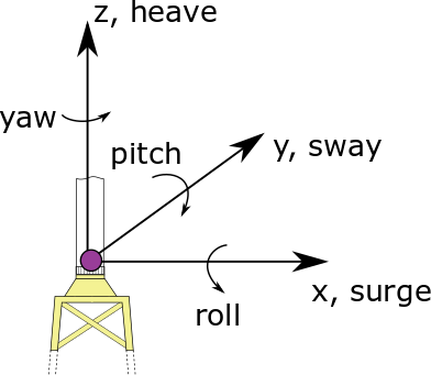
Fig. 4.44 Interface degrees of freedom

ExtPtfm is written in a form that consists of state and output equations. For a linear system, these equations take the following form:

(4.182)\[\begin{split}\begin{aligned} \boldsymbol{\dot{x}}&=\boldsymbol{X}(\boldsymbol{x},\boldsymbol{u}, t) = \boldsymbol{A} \boldsymbol{x}+\boldsymbol{B}\boldsymbol{u} + \boldsymbol{f}_x \\ \boldsymbol{y} &= \boldsymbol{Y}(\boldsymbol{x},\boldsymbol{u}, t) = \boldsymbol{C} \boldsymbol{x}+\boldsymbol{D}\boldsymbol{u} + \boldsymbol{f}_y \end{aligned}\end{split}\]

where \(\boldsymbol{x}\) is the state vector, \(\boldsymbol{u}\) the input vector, and \(\boldsymbol{y}\) the output vector of the module. The input vector of the module is the motion of the interface node, \(\boldsymbol{u}=[\boldsymbol{x}_1, \boldsymbol{\dot{x}}_1, \boldsymbol{\ddot{x}}_1]^t\), whereas the output vector is the coupling load at the interface node, \(\boldsymbol{y}=[\boldsymbol{f}_{C}]^t\). The state vector consists of the motions and velocities of the CB modes, \(\boldsymbol{x}=[\boldsymbol{x}_2, \boldsymbol{\dot{x}}_2]^t\). The dimensions of each vector are: \(\boldsymbol{x}(2n_\text{CB}\times 1)\), \(\boldsymbol{u} (18\times 1)\), \(\boldsymbol{y} (6\times 1)\).

Eq. (4.181) is rewritten in the state-space form of Eq. (4.182) as follows. The second block row of (4.181) is developed to isolate \(\boldsymbol{\ddot{x}}_2\). Using \(\boldsymbol{M}_{r22}=\boldsymbol{I}\) and reintroducing the damping matrix for completeness gives:

(4.183)\[\begin{aligned} \boldsymbol{\ddot{x}}_2=\boldsymbol{f}_{r2}-\boldsymbol{M}_{r12}^t\boldsymbol{\ddot{x}}_1-\boldsymbol{K}_{r22} \boldsymbol{x}_2 -\boldsymbol{C}_{r12}^t\boldsymbol{\dot{x}}_1 -\boldsymbol{C}_{r22}\boldsymbol{\dot{x}}_2 \end{aligned}\]

The matrices of the state-space relation from Eq. (4.182) are then directly identified as ([ep-BSA+20]):

\[\begin{split}\begin{aligned} \boldsymbol{A}= \begin{bmatrix} \boldsymbol{0} & \boldsymbol{I}\\ -\boldsymbol{K}_{r22} & -\boldsymbol{C}_{r22}\\ \end{bmatrix} ,\qquad \boldsymbol{B}= \begin{bmatrix} \boldsymbol{0}& \boldsymbol{0}& \boldsymbol{0}\\ \boldsymbol{0}& -\boldsymbol{C}_{r12}^t& -\boldsymbol{M}_{r12}^t \\ \end{bmatrix} ,\qquad \boldsymbol{f}_x= \begin{bmatrix} \boldsymbol{0} \\ \boldsymbol{f}_{r2}\\ \end{bmatrix} \end{aligned}\end{split}\]

Isolating \(\boldsymbol{f}_{C}\) from the first block row of Eq. (4.181) and using the expression of \(\boldsymbol{\ddot{x}}_2\) from Eq. (4.183) leads to:

\[\begin{split}\begin{aligned} \boldsymbol{f}_{C} =& \boldsymbol{f}_{r1} - \boldsymbol{M}_{r11}\boldsymbol{\ddot{x}}_1 - \boldsymbol{C}_{r11}\boldsymbol{\dot{x}}_1 - \boldsymbol{C}_{r12}\boldsymbol{\dot{x}}_2 - \boldsymbol{K}_{r11}\boldsymbol{x}_1 \nonumber\\ &- \boldsymbol{M}_{r12} (\boldsymbol{f}_{r2}-\boldsymbol{M}_{r12}^t\boldsymbol{\ddot{x}}_1 -\boldsymbol{C}_{r12}^t\boldsymbol{\dot{x}}_1 -\boldsymbol{C}_{r22}\boldsymbol{\dot{x}}_2-\boldsymbol{K}_{r22} \boldsymbol{x}_2)\end{aligned}\end{split}\]

The matrices of for the output \(\boldsymbol{y}\) are then identified as ([ep-BSA+20]):

\[\begin{split}\begin{aligned} \boldsymbol{C}&= \begin{bmatrix} \boldsymbol{M}_{r12}\boldsymbol{K}_{r22} & \boldsymbol{M}_{r12}\boldsymbol{C}_{r22}-\boldsymbol{C}_{r12}\\ \end{bmatrix} ,\qquad \qquad \boldsymbol{f}_y= \begin{bmatrix} \boldsymbol{f}_{r1} - \boldsymbol{M}_{r12}\boldsymbol{f}_{r2}\\ \end{bmatrix} \\ \boldsymbol{D}&= \begin{bmatrix} -\boldsymbol{K}_{r11} & -\boldsymbol{C}_{r11} + \boldsymbol{M}_{r12}\boldsymbol{C}_{r12}^t & -\boldsymbol{M}_{r11}+\boldsymbol{M}_{r12}\boldsymbol{M}_{r12}^t \\ \end{bmatrix} \end{aligned}\end{split}\]

All the block matrices and vectors labeled with “r” are provided to the module via an input file. At a given time step, the loads, \(\boldsymbol{f}_r(t)\), are computed by linear interpolation of the loads given in the input file, and the state equation, , is solved for \(\boldsymbol{x}\) with the outputs returned to the glue code of OpenFAST.

The glue code can also perform the linearization of the full system at a given time or operating point, using the Jacobians of the state equations of each module. Since the formulation of ExtPtfm is linear, the Jacobian of the state and output equations, with respect to the states and inputs of the module, are:

\[\begin{aligned} \frac{\partial \boldsymbol{X}}{\partial \boldsymbol{x}} = \boldsymbol{A} ,\quad \frac{\partial \boldsymbol{Y}}{\partial \boldsymbol{x}} = \boldsymbol{C} ,\quad \frac{\partial \boldsymbol{X}}{\partial \boldsymbol{u}} = \boldsymbol{B} ,\quad \frac{\partial \boldsymbol{Y}}{\partial \boldsymbol{u}} = \boldsymbol{D} \end{aligned}\]

The linearization of ExtPtfm was implemented in the module, but some work remains to be done at the glue-code (OpenFAST) level to allow for full system linearization.