6.1.6.6. Performance Profiling and Tuning
A major focus of the OpenFAST team is performance-profiling and optimization of the OpenFAST software with the goal of improving time-to-solution performance for the most computationally expensive use cases. The process generally involves initial profiling and hotspot analysis, then identifying specific subroutines to target for optimization in the physics modules and glue-codes.
A portion of this work was supported by Intel® through its designation of NLR as an Intel® Parallel Computing Center (IPCC).
The procedures, findings, and recommended programming practices are presented here. This is a working document and will be updating as additional studies are completed.
6.1.6.6.1. High-performance programming techniques
Being a compiled language designed for scientific and engineering applications, Fortran is well suited for producing very efficient code. However, the process of tuning code requires developers to understand the language as well as the tools available (compilers, performance libraries, etc) in order to generate the highest performance. This section identifies programming patterns to use Fortran and the Intel® Fortran compiler effectively. Developers should also reference the Intel® Fortran compiler documentation regarding optimization, in general, and especially the sections on automatic vectorization and coarrays.
6.1.6.6.1.1. Optimization report
When evaluating compiler optimization performance in a complex software, timing tests alone are not a good indication for the compiler’s ability to optimize particular lines of code. For low-level information on the compilers attempts in optimization, developers should generate optimization reports to get line-by-line reporting on various metrics such as vectorization, parallelization, memory and cache usage, threading, and others. Developers should refer to the Intel® Fortran compiler documentation on optimization reports.
For Linux and macOS, the OpenFAST CMake configuration has compiler
flags for generating optimization reports available but commented
in the set_fast_intel_fortran_posix macro in openfast/cmake/OpenfastFortranOptions.cmake.
Primarily, the qopt-report-phase and qopt-report flags should
be used. See the optimization report options documentation
for more information on additional flags and configurations.
With compiler flags correctly configured, the copmiler will output
files with the extension .optrpt alongside the intermediate compile
artifacts like .o files. The compile process will state that
additional files are being generated:
ifort: remark #10397: optimization reports are generated in *.optrpt files in the output location
And the additional files should be located in the corresponding
CMakeFiles directory for each compile target. For example,
the optimization report for the VersionInfo module in OpenFAST
are at:
>> ls -l openfast/build/modules/version/CMakeFiles/versioninfolib.dir/src/
-rw-r--r--  2740 May 12 23:10 VersionInfo.f90.o
-rw-r--r--     0 May 12 23:10 VersionInfo.f90.o.provides.build
-rw-r--r--   668 May 12 23:10 VersionInfo.f90.optrpt
6.1.6.6.1.2. Operator Strength Reduction
Each mathematical operation has an effective “strength”, and some operations can be equivalently represented as a combination of multiple reduced-strength operations that have better performance than the original. As part of the code optimization step, compilers may be able to identify areas where a mathetical operation’s strength can be reduced. Compilers are not able to optimize all expensive operations. For example, cases where a portion of an expensive mathematical operation is a variable contained in a derived data type are frequently skipped. Therefore, it is recommended that expensive subroutines be profiled and searched for possible strength reduction opportunities.
A concrete example of operator strength reduction is in dividing many elements of an array by a constant.
module_type%scale_factor = 10.0

do i = 1
  if array(i) < 30.0
    array(i) = array(i) / module_type%scale_factor
  end if
end do
In this case, a multiplication of real numbers is less expensive than a division of real numbers. The code can be factored so that the inverse of the scale factor is computed outside of the loop and the mathematical operation in the loop is converted to a multiplication.
module_type%scale_factor = 10.0
inverse_scale_factor = 1.0 / module_type%scale_factor

do i = 1
  if array(i) < 30.0
    array(i) = array(i) * inverse_scale_factor
  end if
end do
6.1.6.6.1.3. Coarrays
Coarrays are a feature introduced to the Fortran language in the 2008 standard to provide language-level parallelization for array operations in a Single Program, Multiple Data (SPMD) programming paradigm. The Fortran standard leaves the method of parallelization up to the compiler, and the Intel® Fortran compiler uses MPI.
Coarrays are used to split an array operation across multiple copies of the program. The copies are called “images”. Each image has its own local variables, plus a portion of any coarrays as shared variables. A coarray can be thought of as having extra dimensions, referred to as “codimensions”. A single image (typically the 1-th index) controls the I/O and problem setup, and images can read from memory in other images.
For operations on large arrays such as constructing a super-array from many sub-arrays (as in the construction of a Jacobian matrix), the coarray feature of Fortran 08 can parallelize the procedure improving overall computational efficiency.
6.1.6.6.1.4. Data modeling and access rules
Fortran represents arrays in column-major order. This means that a multidimensional array is represented in memory with column elements being adjacent. If a given element in an array is at a location in memory, one element before in memory corresponds to the element above it in its column.
In order to make use of the single instruction, multiple data
features of modern processors, array construction and access
should happen in column-major order. That is, loops should loop
over the left-most index quickest. Slicing should occur with
the : also on the left-most index when possible.
With this in mind, data should be represented as structures of arrays rather than arrays of structures. Concretely, this means that data types within OpenFAST should contain the underlying arrays and arrays should generally contain only numeric types.
The short program below displays the distance in memory in units of bytes between elements of an array and neighboring elements.
program memloc

implicit none

integer(kind=8), dimension(3, 3) :: r, distance_up, distance_left

! Take the element values as their "ID"
! r(row, column)
r(1,:) = (/ 1, 2, 3 /)
r(2,:) = (/ 4, 5, 6 /)
r(3,:) = (/ 7, 8, 9 /)
print *, "Reference array:"
call pretty_print_array(r)

! Compute the distance between matrix elements. Inputs to the `calculate_distance` function
! are indices for elements in the equation loc(this_element) - loc(other_element)
distance_up(1,:) = (/ calculate_distance( 1,1 , 1,1), calculate_distance( 1,2 , 1,2), calculate_distance( 1,3 , 1,3) /)
distance_up(2,:) = (/ calculate_distance( 2,1 , 1,1), calculate_distance( 2,2 , 1,2), calculate_distance( 2,3 , 1,3) /)
distance_up(3,:) = (/ calculate_distance( 3,1 , 2,1), calculate_distance( 3,2 , 2,2), calculate_distance( 3,3 , 2,3) /)
print *, "Distance in memory (bytes) for between an element and the one above it (top row zeroed):"
call pretty_print_array(distance_up)

distance_left(1,:) = (/ calculate_distance( 1,1 , 1,1), calculate_distance( 1,2 , 1,1), calculate_distance( 1,3 , 1,2) /)
distance_left(2,:) = (/ calculate_distance( 2,1 , 2,1), calculate_distance( 2,2 , 2,1), calculate_distance( 2,3 , 2,2) /)
distance_left(3,:) = (/ calculate_distance( 3,1 , 3,1), calculate_distance( 3,2 , 3,1), calculate_distance( 3,3 , 3,2) /)
print *, "Distance in memory (bytes) for between an element and the one to the its left (first column zeroed):"
call pretty_print_array(distance_left)

contains

integer(8) function calculate_distance(c1, r1, c2, r2)

    integer, intent(in) :: c1, r1, c2, r2
    calculate_distance = loc(r(c1, r1)) - loc(r(c2, r2))

end function

subroutine pretty_print_array(array)

    integer(8), dimension(3,3), intent(in) :: array
    print *, "["
    print '(I4, I4, I4)', array(1,1), array(1,2), array(1,3)
    print '(I4, I4, I4)', array(2,1), array(2,2), array(2,3)
    print '(I4, I4, I4)', array(3,1), array(3,2), array(3,3)
    print *, "]"

end subroutine

end program
6.1.6.6.2. Optimization Studies
This section describes specific efforts to profile sections of OpenFAST and improve performance with the Intel® compiler suite.
6.1.6.6.2.1. BeamDyn Performance Profiling and Optimization (IPCC Year 1 and 2)
The general mechanisms identified for performance improvements in OpenFAST were:
Intel® compiler suite and Intel® Math Kernel Library (Intel® MKL)
Algorithmic improvements
Memory-access optimization enabling more efficient cache usage
Data type alignment allowing for SIMD vectorization
Multithreading with OpenMP
To establish a path forward with these options, OpenFAST was first profiled with Intel® VTune™ Amplifier to get a clear breakdown of time spent in the simulation. Then, the optimization report generated from the Intel® Fortran compiler was analyzed to determine areas that were not autovectorized. Finally, Intel® Advisor was used to highlight areas of the code that the compiler identified as potentially improved with multithreading.
Two OpenFAST test cases have been chosen to provide meaningful and realistic timing benchmarks. In addition to real-world turbine and atmospheric models, these cases are computationally expensive and expose the areas where performance improvements would make a difference.
5MW_Land_BD_DLL_WTurb
Download case files here.
The physics modules used in this case are:
BeamDyn
InflowWind
AeroDyn 15
ServoDyn
This is a land based Jonkman 5-MW (formerly called the NREL 5-MW) turbine simulation using BeamDyn as the structural module. It simulates 20 seconds with a time step size of 0.001 seconds and executes in 3m 55s on NLR’s former Peregrine supercomputer (retired).
5MW_OC4Jckt_DLL_WTurb_WavesIrr_MGrowth
Download case files here.
This is an offshore, fixed-bottom Jonkman 5-MW (formerly called the NREL 5-MW) turbine simulation with the majority of the computational expense occurring in the HydroDyn wave-dynamics calculation.
The physics modules used in this case are:
ElastoDyn
InflowWind
AeroDyn 15
ServoDyn
HydroDyn
SubDyn
It simulates 60 seconds with a time step size of 0.01 seconds and executes in 20m 27s on NLR’s former Peregrine supercomputer (retired).
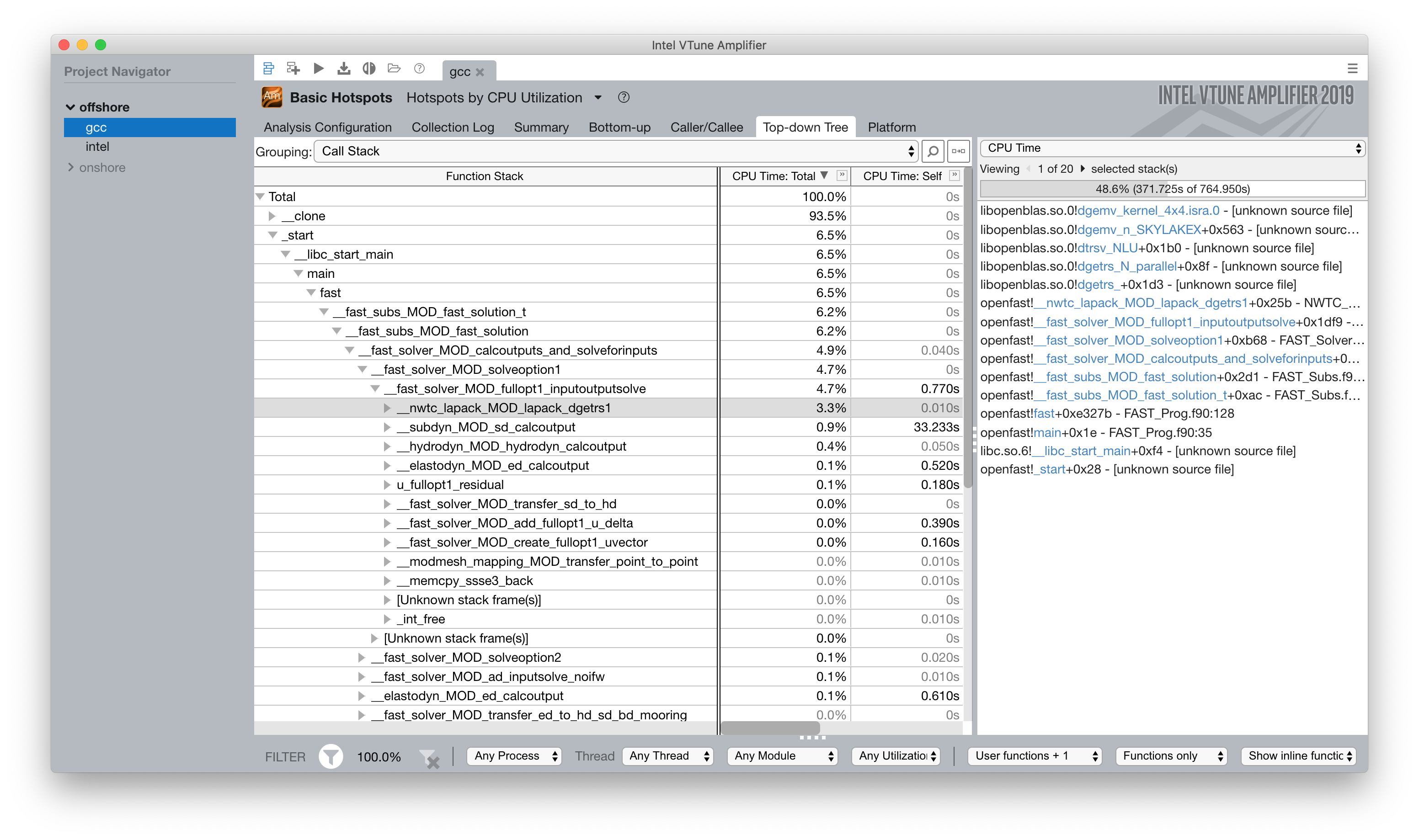
6.1.6.6.2.1.1. Profiling
The OpenFAST test cases were profiled with Intel® VTune™ Amplifier to
identify performance hotspots. Being that the two test cases exercise
difference portions of the OpenFAST software, different hotspots were
identified. In all cases and environment settings, the majority of the
CPU time was spent in fast_solution loop which is a high-level subroutine
that coordinates the solution calculation from each physics module.
6.1.6.6.2.1.1.1. LAPACK
In the offshore case, the LAPACK usage was identified as a performance load.
Within the fast_solution loop, the calls to the LAPACK function dgetrs
consume 3.3% of the total CPU time.
6.1.6.6.2.1.1.2. BeamDyn
While BeamDyn provides a high-fidelity blade-response calculation, it is a
computationally expensive module. Initial profiling highlighted the
bd_elementmatrixga2 subroutine as a hotspot. However, initial
attempts to improve performance in BeamDyn revealed needs for algorithmic
improvements and refinements to the module’s data structures.
6.1.6.6.2.1.2. Results
Though work is ongoing, OpenFAST time-to-solution performance has improved and the performance potential is better understood.
Some keys outcomes from the first year of the IPCC project are as follows:
Use of Intel® compiler and MKL library provides dramatic speedup over GCC and LAPACK
Additional significant gains are possible through MKL threading for offshore simulations
Offshore-wind-turbine simulations are poorly load balanced across modules
Land-based-turbine configuration better balanced
OpenMP Tasks are employed to achieve better load-balancing
OpenMP module-level parallelism provides significant, but limited speed up due to imbalance across different module tasks
Core algorithms need significant modification to enable OpenMP and SIMD benefits
Tuning the Intel® tools to perform best on NLR’s hardware and adding high level multithreading yielded a maximum 3.8x time-to-solution improvement for one of the benchmark cases.
6.1.6.6.2.1.2.1. Speedup - Intel® Compiler and MKL
By employing the standard Intel® developer tools tech stack, a performance improvement over GNU tools was demonstrated:
Compiler |
Math Library |
5MW_Land_BD_DLL_WTurb |
5MW_OC4Jckt_DLL_WTurb_WavesIrr_MGrowth |
|---|---|---|---|
GNU |
LAPACK |
2265 s (1.0x) |
673 s (1.0x) |
Intel® 17 |
LAPACK |
1650 s (1.4x) |
251 s (2.7x) |
Intel® 17 |
MKL |
1235 s (1.8x) |
— |
Intel® 17 |
MKL Multithreaded |
722 s (3.1x) |
— |
6.1.6.6.2.1.2.2. Speedup - OpenMP at FAST_Solver
A performance improvement was domenstrated by adding OpenMP directives to the
FAST_Solver module. Although the solution scheme is not well balanced,
parallelizing mesh mapping and calculation routines resulted in the following
speedup:
Compiler |
Math Library |
5MW_Land_BD_DLL_WTurb |
5MW_OC4Jckt_DLL_WTurb_WavesIrr_MGrowth |
|---|---|---|---|
Intel® 17 |
MKL - 1 thread |
1073 s (2.1x) |
100 s (6.7x) |
Intel® 17 |
MKL - 8 threads |
597 s (3.8x) |
— |
6.1.6.6.2.1.3. Ongoing Work
The next phase of the OpenFAST performance improvements are focused in two key areas:
Implementing the outcomes from previous work throughout OpenFAST modules and glue codes
Preparing OpenFAST for efficient execution on Intel®’s next generation platforms
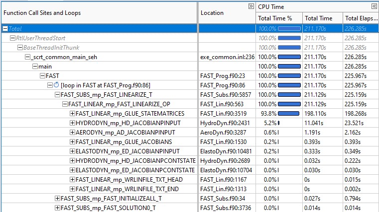
6.1.6.6.2.2. Linearization routine profiling
As a portion of the ARPA-E WEIS project, the linearization capability within OpenFAST has been profiled in an effort to characterize the performance and current bottlenecks. This work specifically targetted the linearization routines within the FAST Library, primarily in FAST_Lin.f90, as well as the routines constructing the Jacobian matrices within individual physics modules. Because these routines require constructing large matrices, this is a computationally intensive process with a high rate of memory access.
A high-level flow of data in the linearization algorithm in the
FAST_Linearize_OP subroutine is given below.
        graph TD;
  D[Construct Module Jacobian]-->A[Calculate Module OP];
  A[Calculate Module OP]-->B[Construct Glue Code Jacobians];
  A[Calculate Module OP]-->C[Construct Glue Code State Matrices];
Each enabled physics module constructs module-level matrices in their respective
<Module>_Jacobian and <Module>_GetOP routines, and the collection of these
are assembled into global matrices in Glue_Jacobians and Glue_StateMatrices.
In a top-down comparison of total CPU time in FAST_Linearize_OP, we see that
the construction of the glue-code state matrices is the most expensive step.
The HydroDyn Jacobian computation also stands out relative to other module
Jacobian computations.
The Jacobian and state matrices are sized based on the total number of inputs, outputs, and continuous states. Though the size varies, these matrices generally contain thousands of elements in each dimension and are mostly zeroes. That is to say, the Jacobian and state matrices are large and sparse. To reduce the overhead of memory allocation and access, a sparse matrix representation is recommended.