4.9.3. ElastoDyn Theory
Note this document is work in progress and is greatly incomplete. This documentation was started to document some code changes to the tail furl and rotor furl part of ElastoDyn. Please refer to the different ressources provided in Section 4.9 for additional documents.
4.9.3.1. Notations
Points
The following (partial) list of points are defined by ElastoDyn:
Z: the platform reference pointO: the tower-top/base plate pointW: the specified point on the tail-furl axisI: the tail boom center of massJ: the tail fin center of mass
Bodies
The following (partial) list of bodies are defined by ElastoDyn:
E: the earth/inertial frameX: the platform bodyN: the nacelle bodyA: the tail-furl body
4.9.3.2. Kinematics
ElastoDyn computes the position, velocity and accelerations of key points of the structure, starting from the platform reference point Z and going up in the structure.
The different position vectors are available in the data stucture RtHSdat.
For instance, the global position of point J is given by:
The translational displacement vector (how much a point has moved compared to its reference position) is calculated as follows: \(\boldsymbol{r}_J-\boldsymbol{r}_{J,\text{ref}}\).
The coordinate systems of ElastoDyn are stored in the variable CoordSys.
The orientation matrix of a given coordinate system can be formed using the unit vectors (assumed to be column vectors) of a given coordinate system expressed in the inertial frame.
For instance for the tailfin coordinate system:
Angular velocities are stored in variables RtHSdat%AngVelE* with respect to the initial frame (“Earth”, E).
For instance, the angular velocity of the tail-furl body (body A) is:
where \(\boldsymbol{\omega}_{N/X}=\boldsymbol{\omega}_{B/X}+\boldsymbol{\omega}_{N/B}\)
Linear (translational) velocities of the different points are found in the variables RtHSdat%LinVelE*, and are computed based on Kane’s partial velocities (which are Jacobians of the velocity with respect to the time derivatives of the degrees of freedom).
For instance, the linear velocity of point J is computed as:
where the Jacobians \(\frac{\partial v_J}{\partial \dot{q}_j}\) are stored in RtHSdat%PLinVelEJ(:,0)
Translational accelerations are computed as the sum of contribution from the first and second time derivatives of the degrees of freedom. For instance, the acceleration of point J is computed as:
where \(\frac{\partial a_J}{\partial \dot{q}_j}\) are stored in RtHSdat%PLinVelEJ(:,1)
Angular accelerations requires similar computations currently not documented.
4.9.3.3. Rotor and tail furl
The user can select linear spring and damper models, together with up- and down-stop springs, and up- and down-stop dampers.
The torque applied from the linear spring and damper is:
where \(\theta\) is the degree of freedom (rotor or tail furl),
\(k\) is the linear spring constant (RFrlSpr or TFrlSpr)
\(d\) is the linear damping constant (RFrlDmp or TFrlDmp).
The up-/down- stop spring torque is defined as:
where
\(k_{US}\) is the up-stop spring constant (RFrlUSSpr or TFrlUSSpr),
\(\theta_{k_{US}}\) is the up-stop spring angle (RFrlUSSP or TFrlUSSP),
and similar notations are used for the down-stop spring.
The up-/down- stop damping torque is defined as:
where similar nnotations are used. The total moment on the given degree of freedom is:
4.9.3.4. Yaw-friction model
A yaw-friction model is implemented in ElastoDyn based on a Coulomb-viscous approach. The yaw-friction moment as a function of yaw rate (\(\omega\)) is shown below in Fig. 4.48
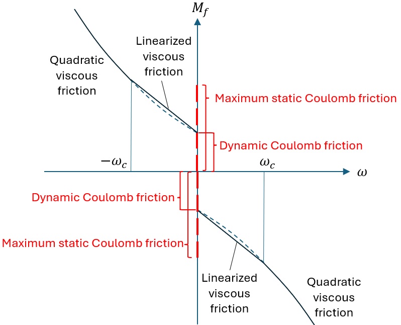
Fig. 4.48 Yaw-friction model
When YawFrctMod = 1, the maximum static or dynamic Coulomb friction does not depend on the external load on the yaw bearing. The yaw-friction torque \(M_f\) can be calculated as follows.
If \(\omega\neq0\), we have dynamic friction of the form
where \(\bar{D}\) is the effective yaw-bearing diameter and \(\mu_d\) is the dynamic Coulomb friction coefficient. Their product, \(\mu_d\bar{D}\), is specified in the input file through M_CD. The first term on the right-hand side is the dynamic Coulomb friction.
The viscous friction, \(M_{f,vis}\), is of the form
or
where \(\sigma_v\) and \(\sigma_{v2}\) are the linear and quadratic viscous friction coefficients and \(\omega_c\) is the cutoff yaw rate below which viscous friction is linearized. Setting \(\omega_c=0\) disables the linearization of viscous friction.
If \(\omega=0\) and \(\dot{\omega}\neq 0\), we have a slightly modified dynamic Coulomb friction of the form
where \(M_z\) is the external yaw torque. If \(\omega=0\) and \(\dot{\omega}=0\), we have static Coulomb friction of the form
where \(\mu_s\) is the static Coulomb friction coefficient. The product \(\mu_s\bar{D}\) is specified in the input file through M_CSmax.
When YawFrctMod = 2, the maximum static or dynamic Coulomb friction depends on the external load on the yaw bearing, with proportional contributions from \(\left|F_z\right|\), the magnitude of the bearing axial load, if \(F_z<0\), from the bearing shear force magnitude, \(\sqrt{F_x^2+F_y^2}\), and from the bearing bending moment magnitude, \(\sqrt{M_x^2+M_y^2}\).
If \(\omega\neq0\), we have dynamic friction of the form
where \(M_{f,vis}\) is defined in the same way as when YawFrctMod = 1. The product \(\mu_{df}\bar{D}\) and \(\mu_{dm}\) are specified in the input file through M_FCD and M_MCD, respectively.
If \(\omega=0\) and \(\dot{\omega}\neq 0\), we have a modified dynamic Coulomb friction of the form
If \(\omega=0\) and \(\dot{\omega}=0\), we have static Coulomb friction of the form
where the product \(\mu_{sf}\bar{D}\) and \(\mu_{sm}\) are specified in the input file through M_FCSmax and M_MCSmax, respectively.
The static ‘stiction’ (where the static contribution exceeds the dynamic Coulomb friction) is only applied if both the yaw rotational velocity and acceleration at the current time-step are zero. The static portion of the friction is omitted if the rotational acceleration is not null. This is to account for the fact that a ‘warm’ joint may not feel stiction when crossing through zero velocity in a dynamic sense [ed-HWS23]. When \(\omega=0\), the yaw-bearing static or dynamic friction is formulated such that the frictional resistance opposes the external applied moment, \(M_z\), without overcoming it.
4.9.3.5. Blade pitch dynamics
Prior to OpenFAST v5, the blade pitch angles were either fixed or prescribed based on the pitch command from ServoDyn. The blade root pitch velocity and acceleration were always zero despite the pitch angle potentially changing following ServoDyn pitch command. There was also no pitch moment due to blade pitch inertia if the blades are modeled in ElastoDyn. Note that when BeamDyn was used to model the blades, only the blade root nodes had zero pitch velocity and acceleration. The pitch inertia and twisting of the rest of the blades following the root node were still accounted for, partially capturing the blade pitch dynamics.
In OpenFAST v5, new blade pitch degrees of freedom, PitchDOF, are introduced in ElastoDyn. By setting PitchDOF to true, blade pitching can now be simulated dynamically in ElastoDyn. To use this feature, users need to provide the moments of inertia of the pitch actuators/bearings about the pitch axis through the new PBrIner(I) inputs added to the ElastoDyn input file. If the blades are also modeled in ElastoDyn instead of BeamDyn, the total moments of inertia of the undeflected blades about the pitch axis must also be provided through the new BlPIner(I) inputs. Note that because ElastoDyn does not model blade twisting, it is not necessary to specify distributed blade pitch inertia. Furthermore, the effective blade pitch moments of inertia during the simulation might be higher than BlPIner(I) due to additional contributions coming from blade bending. When ElastoDyn is used to model the blades, PBrIner(I) and BlPIner(I) are simply added together to obtain the total pitch moment of inertia needed in the equations of motion. The results from the simulation will be the same as long as the sum of PBrIner(I) and BlPIner(I) remains unchanged. When BeamDyn is used to model the blades, BlPIner(I) is ignored because the distributions of pitch moment of inertia along the blades are considered in BeamDyn, which also models blade twisting. It is, however, still necessary to have realistic values for PBrIner(I) in ElastoDyn. Setting PBrIner(I) to zero or close to zero will result in numerical issues in ElastoDyn.
When PitchDOF is true, the blade root pitch angles are solved dynamically instead of being prescribed. In this case, a pitch actuator torque is computed by ServoDyn for each blade as
BlPitchMom = - PitSpr * ( BlPitch - BlPitchCom ) - PitDamp * ( BlPRate - BlPRateCom )
The pitch actuator stiffness/spring constant PitSpr and damping PitDamp for each blade are both defined in the ServoDyn input file. This actuator torque is applied to the blade at the root. An equal but opposite torque is applied to the rotor hub. The pitch command BlPitchCom and pitch rate command BlPRateCom are not used by ElastoDyn directly when PitchDOF is true. (ServoDyn will compute and output pitch actuator torques regardless of whether PitchDOF is true or false in ElastoDyn. However, in the latter case, the actuator torques are simply not used.)
When active blade pitch control is on in ServoDyn, BlPitchCom is computed by the turbine controller. When active blade pitch control is off (PCMode=0 or during t<TPCOn when PCMode>0), BlPitchCom is given by the neutral blade pitch position PitNeut(I) in the ServoDyn input file. Finally, during pitch maneuver, BlPitchCom approaches the final pitch position at a constant rate given by PitManRat(I) in the ServoDyn input file.
In addition to pitch position commands, pitch rate commands BlPRateCom are also added to ServoDyn. Currently, BlPRateCom is only available with DLL controllers (PCMode=5) or during override pitch maneuvers. During normal operation, the pitch rate commands are estimated using finite differencing based on the pitch set points from two consecutive controller steps. During pitch maneuvers, the pitch rate command is simply set to PitManRat(I) in the ServoDyn input file until the final pitch position is reached. BlPRateCom is zero when PCMode is 0, 3, or 4 or after the pitch maneuver is completed.
When PitchDOF is true in ElastoDyn, the following ServoDyn settings are recommended:
When using a DLL controller (
PCMode=5), setBPCutoffto an appropriate value (on the order of 1 Hz depending on the turbine) to avoid discontinuities in the pitch-rate command. This can help reduce large fluctuations in the actuator torque. The same low-pass filter is applied to both pitch command and pitch rate command.For consistency with the pitch rate command estimated using finite differencing, set
DLL_Rampto true. This can reduce small jitters in the actuator moment whenDLL_DTis larger than the simulation time step.Finally, the pitch actuator stiffness and damping must be set appropriately to obtain a reasonable time constant (on the order of a quarter of a second) and damping ratio (about 0.7). Higher
PitSpr(I)andPitDamp(I)will require a smaller time step for numerical stability. To achieve a given damped periodTdand damping ratiozeta, the following equations can be used to obtain initial estimates ofPitSpr(I)andPitDamp(I):
PitSpr = 4 * pi^2 * ( PBrIner + BlPIner ) / ( Td^2 * ( 1 - zeta^2 ) )
PitDamp = 2 * zeta * sqrt( PitSpr * ( PBrIner + BlPIner ) )
When PitchDOF is true, the following new output channels from ElastoDyn become available:
BldPRate1- blade 1 pitch rate (deg/s)BldPRate2- blade 2 pitch rate (deg/s)BldPRate3- blade 3 pitch rate (deg/s)BldPAcc1- blade 1 pitch acceleration (deg/s^2)BldPAcc2- blade 2 pitch acceleration (deg/s^2)BldPAcc3- blade 3 pitch acceleration (deg/s^2)
These output channels are valid only if PitchDOF is true with positive values toward the feathered position.
If PitchDOF is false in ElastoDyn, OpenFAST will function as before with the blade root pitch angles either fixed to the initial positions defined in ElastoDyn when ServoDyn is disabled or set to the pitch commands from ServoDyn. Setting PitchDOF to false does not mean the blade pitch angles will be constant. PBrIner(I) and BlPIner(I) in the ElastoDyn input file are both ignored when PitchDOF is false. The pitch actuator torques from ServoDyn are also ignored by ElastoDyn. Finally, note that the initial blade pitch positions specified in ElastoDyn will be superseded by PitNeut(I) in ServoDyn if ServoDyn is enabled but active blade pitch control is off (PCMode=0 or during t<TPCOn when PCMode>0).
Usage guidance
The effect of enabling PitchDOF on blade root loads tends to be more significant when the blades are modeled in ElastoDyn. This is because ElastoDyn will entirely ignore the blade pitch inertia otherwise. When the blades are modeled in BeamDyn, the effect tends to be less significant because blade pitch inertia (except that of the root node) and blade twisting will always be accounted for. In this case, enabling PitchDOF in ElastoDyn allows the pitch inertia of the entire blade, including that of the root node, to be included in the dynamics.
Furthermore, the impact of PitchDOF tends to be more significant after sudden starts or stops in blade pitching. For example, this can happen during normal operation when the blade pitch angle saturates (if the pitch command is not low-pass filtered as suggested above) or during emergency shutdown when the blades need to quickly pitch to the feathered position and stop. In these situations, enabling PitchDOF allows OpenFAST to capture the large pitch moments at the blade roots that would otherwise be missed if the blades are modeled in ElastoDyn. Alternatively, if the blades are modeled in BeamDyn, it prevents discontinuous pitch rates at the blade roots and can help smooth out large fluctuations in the root moments immediately following the impulsive start or sudden stop.
4.9.4. Developer notes
Internal coordinate systems
The different coordinate systems of ElastoDyn are stored in the variable CoordSys.
The coordinate systems used internally by ElastoDyn are using a different convention than the OpenFAST input/output coordinate system.
For instance, for the coordinate system of the nacelle, with unit axes noted \(x_n,y_n,z_n\) in OpenFAST, and \(d_1,d_2,d_3\) in ElastoDyn, the following conversions apply: \(d_1 = x_n\), \(d_2 =z_n\) and \(d_3 =-y_n\).
The following (partial) list of coordinate systems are defined internally by ElastoDyn:
z : inertial coordinate system
a : tower base coordinate system
t : tower-node coordinate system (one per node)
d : nacelle coordinate system
c : shaft-tilted coordinate system
rf : rotor furl coordinate system
tf : tail furl coordinate system
g : hub coordinate system